Linear 2nd order ODE with constant coefficients

Homogeneous:

\[{y^{\prime\prime}} + A{y^{\prime}} + By = 0\]

Solution:

\[y = {c_1}{y_1} + {c_2}{y_2}\]

in which, \({y_1}\) and \({y_2}\) are two independent solutions of the homogeneous ODE.

The basic method to solve this ODE is to try \(y = {e^{rt}}\). Plug in and we can get

\[{r^2}{e^{rt}} + Ar{e^{rt}} + B{e^{rt}} = 0 \to {r^2} + Ar + B = 0\]

Case 1: two different real roots

\[y = {c_1}{e^{{r_1}t}} + {c_2}{e^{{r_2}t}}\]

Case 2: complex roots \(r = a \pm bi\)

\[y = {e^{a + bi}} = {e^{at}}\cos \left( {bt} \right) + {e^{at}}\sin \left( {bt} \right)i\]

Theorem: If \(u + iv\) is a solution to \({y^{\prime\prime}} + A{y^{\prime}} + By = 0\), then \(u,{\kern 1pt} {\kern 1pt} {\kern 1pt} v\) are real solutions.

Proof:

\[{\left( {u + iv} \right)^{\prime\prime}} + A{\left( {u + iv} \right)^{\prime}} + B\left( {u + iv} \right) = 0\]

\[{u^{\prime\prime}} + A{u^{\prime}} + Bu + i\left( {{u^{\prime\prime}} + A{u^{\prime}} + Bu} \right) = 0\]

Thus, both the real part and the imaginary part have to be zero and the solution is

\[y = {e^{at}}\left( {{c_1}\cos bt + {c_2}\sin bt} \right)\]

Case 3: two same real roots

If \({y_1}\) is a solution to \({y^{\prime\prime}} + A{y^{\prime}} + By = 0\), there is another solution \(y = {y_1}u\).

Proof:

\[\left\{ \begin{array}{l}
{a^2}\left( {y = {e^{ – at}}u} \right)\\
2a\left( {{y^{\prime}} = – a{e^{ – at}}u + {e^{ – at}}{u^{\prime}}} \right)\\
1 \cdot \left( {{y^{\prime\prime}} = {a^2}{e^{ – at}}u – 2a{e^{ – at}}{u^{\prime}} + {e^{ – at}}{u^{\prime\prime}}} \right)
\end{array} \right.\]

Plus all the three equations and then we get

\[0 = 0 + 0 + {e^{ – at}}{u^{\prime\prime}}\]

\[{e^{ – at}}{u^{\prime\prime}} = 0 \to {u^{\prime\prime}} = 0\]

The most simple form of \(u\) is \(u = {C_1}t + {C_2}\), so that the solution is

\[y = {c_1}{e^{ – at}} + {c_2}{e^{ – at}}t\]

Example:

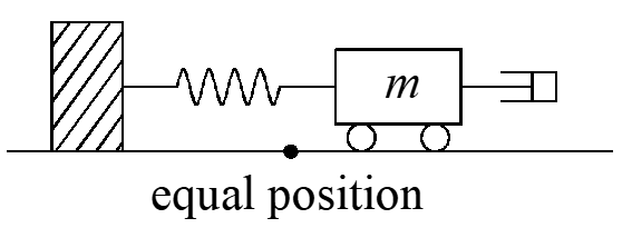
\[m{x^{\prime\prime}} = – kx – c{x^{\prime}} \to {x^{\prime\prime}} + \frac{c}{m}{x^{\prime}} + \frac{k}{m}x = 0\]

ODE with different solutions (two real roots, one double root, complex roots) with the same initial conditions \(y\left( 0 \right) = 1,{y^{\prime}}\left( 0 \right) = 0\)

\[{y^{\prime\prime}} + 4{y^{\prime}} + 3y = 0 \to y = \frac{3}{2}{e^t} – \frac{1}{2}{e^{3t}}\]

\[{y^{\prime\prime}} + 4{y^{\prime}} + 4y = 0 \to y = {e^{ – 2t}} + 2t{e^{ – 2t}}\]

\[{y^{\prime\prime}} + 4{y^{\prime}} + 5y = 0 \to y = {e^{ – 2t}}\left( {\cos t + 2\sin t} \right)\]

The figure of the third equation drawn by Matlab as follow

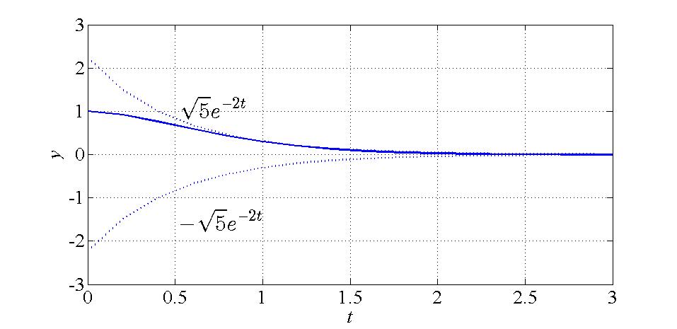
Codes used in figure plotting:

t=0:0.2:3;
plot(t,sqrt(5)*exp(-2*t),':', 'linewidth', 2)
hold on
grid on; 
xlabel('t');
ylabel('y');
plot(t,-sqrt(5)*exp(-2*t),':', 'linewidth', 2);
plot(t,(cos(t)+2*sin(t)).*exp(-2*t), 'linewidth', 2);
set(gca,'FontSize',20,'FontName', 'times new roman');
set(get(gca,'XLabel'),'Fontsize',20, 'FontName','Times New Roman','FontAngle','italic');
set(get(gca,'YLabel'),'Fontsize',20, 'FontName','Times New Roman','FontAngle','italic');

About case 2

In case 2, we only use one of the complex roots \(a + bi\) to form the solution, will the solution be different if written with the other complex root \(a – bi\)? If we use the root root \(a – bi\), then

\[{y_1} = {e^{at}}\cos \left( { – bt} \right), – {y_2} = {e^{at}}\sin \left( { – bt} \right)\]

So, the solutions are the same.

If we just use the two complex roots to write the solution, then the solution can be written as follow where \({c_1}\) and \({c_2}\) can be complex numbers.

\[y = {c_1}{e^{\left( {a + bi} \right)t}} + {c_2}{e^{\left( {a – bi} \right)t}}\]

The real solution is the real part of the above equation.

Method 1: by hack

\[{c_1} = {d_1} + {f_1}i, {c_2} = {d_2} + {f_2}i\]

Method 2: if we want real part of \(u + vi\), then \(v = 0\), that means we just need to see if the equations are the same when changing \(i\) into \(-i\).

\[{c_1}{e^{\left( {a + bi} \right)t}} + {c_2}{e^{\left( {a – bi} \right)t}} \to {\overline c _1}{e^{\left( {a – bi} \right)t}} + {\overline c _2}{e^{\left( {a + bi} \right)t}}\]

If the two are the same, then

\[{c_1} = {\overline c _2},{c_2} = \overline c _1\]

Actually, the second equation is redundant and the same as the first one. Thus, assume \({c_1} = c + di\) and complex conjugate

\[\left( {c + di} \right){e^{\left( {a + bi} \right)t}} + \left( {c – di} \right){e^{\left( {a – bi} \right)t}}\]

In science and engineering, the solutions are often written in this way for application. Change the equation to \({\cos }\) and \({\sin }\):

method 1: hack method

method 2: nicer method

\[{e^{at}}\left[ {c\left( {{e^{ibt}} + {e^{ – ibt}}} \right) + id\left( {{e^{ibt}} – {e^{ – ibt}}} \right)} \right] = {e^{at}}\left[ {2c\cos bt + 2id\sin bt} \right]\]

with the backwards of Euler formula

\[\left\{ \begin{array}{l}
\cos a = \frac{{{e^{ia}} + {e^{ – ia}}}}{2}\\
\sin a = \frac{{{e^{ia}} – {e^{ – ia}}}}{{2i}}
\end{array} \right.\]

In the spring-mass-dashpot system, the equation can be written with circular frequency \( \omega _0\)

\[m{x^{\prime\prime}} + c{x^{\prime}} + kx = 0 \to {y^{\prime\prime}} + 2p{y^{\prime}} + \omega _0^2y = 0\]

Undamped case: \(p = 0\)

\[{y^{\prime\prime}} + \omega _0^2y = 0\]

\[y = {c_1}\cos {\omega _0}t + {c_2}\sin {\omega _0}t = A\cos \left( {{\omega _0}t – \phi } \right)\]

Damped case: \(p < {\omega _0}\) with complex roots

The half “period” of the solution \(\omega _1\), which is called pseudo circular frequency, goes down with the increase of damp \(c\).

\[r = – p \pm \sqrt { – \left( {\omega _0^2 – {p^2}} \right)} = – p \pm \sqrt { – \omega _1^2} \]

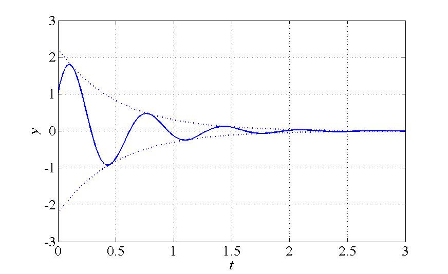
\[y = {e^{ – pt}}\left( {{c_1}\cos {\omega _1}t + {c_2}\sin {\omega _1}t} \right) = A{e^{ – pt}}\cos \left( {{\omega _1}t – \phi } \right)\]

We can see that the amplitude \(A\)and phase lag \(\phi\) depend on the initial conditions, while the \(\omega _1\) only relies on the ODE (damping and spring) with the relationship

\[\omega _1^2 = \omega _0^2 – {p^2}\]

The typical oscillation with damp is figured as follow. The line in dot is the amplitude of the motion.

Theory about homogeneous second-order ODE

To find the solution to \({y^{\prime\prime}} + b{y^{\prime}} + ky = 0\) is to find to independent solutions \({y_1}\) and \({y_1}\), satisfying

\[{y_2} \ne c{y_1},{y_1} \ne {c^{\prime}}{y_2}\]

Then all solutions can be expressed as

\[y = {c_1}{y_1} + {c_2}{y_2}\]

Q1: Why \({c_1}{y_1} + {c_2}{y_2}\) are solutions?

Superposition principle

If \({y_1}\) and \({y_1}\) are solutions to linear homogeneous ODE, then \({c_1}{y_1} + {c_2}{y_2}\) is a solution to the ODE.

Proof:

\[{y^{\prime\prime}} + p{y^{\prime}} + qy = 0 \to {D^2}y + pDy + qy = 0 \to \left( {{D^2} + pD + q} \right)y = 0\]

\({L = {D^2} + pD + q}\) is a linear operator

two laws:

\[\left\{ \begin{array}{l}
L\left( {{u_1} + {u_2}} \right) = L\left( {{u_1}} \right) + L\left( {{u_2}} \right)\\
L\left( {cu} \right) = cL\left( u \right)
\end{array} \right.\]

The proof is very simple and omitted here, you can just expand the left side of the equation in the law and reassemble to the form in the right side.

Proof of superposition with ODE \(Ly = 0\)

\[L\left( {{c_1}{y_1} + {c_2}{y_2}} \right) = L\left( {{c_1}{y_1}} \right) + L\left( {{c_2}{y_2}} \right) = {c_1}L\left( {{y_1}} \right) + {c_2}L\left( {{y_2}} \right) = 0\]

Q2: Why \({c_1}{y_1} + {c_2}{y_2}\) are all solutions?

Assume the initial condition for the ODE is

\[y\left( {{x_0}} \right) = a,{y^{\prime}}\left( {{x_0}} \right) = a\]

So, to find the value of variables \({c_1}\) and \({c_2}\)

\[\left\{ \begin{array}{l}
{c_1}{y_1}\left( {{x_0}} \right) + {c_2}{y_2}\left( {{x_0}} \right) = a\\
{c_1}y_1^{\prime}\left( {{x_0}} \right) + {c_2}y_2^{\prime}\left( {{x_0}} \right) = b
\end{array} \right.\]

The equation set is solvable for \({c_1}\) and \({c_2}\) if the coefficients are invertable

\[\left| {\begin{array}{*{20}{c}}
{{y_1}\left( {{x_0}} \right)}&{{y_2}\left( {{x_0}} \right)}\\
{y_1^{\prime}\left( {{x_0}} \right)}&{y_2^{\prime}\left( {{x_0}} \right)}
\end{array}} \right| \ne 0\]

Wronskian

\[W\left( {{y_1},{y_2}} \right) = \left| {\begin{array}{*{20}{c}}
{{y_1}}&{{y_2}}\\
{y_1^{\prime}}&{y_2^{\prime}}
\end{array}} \right|\]

Theorem

If \({y_1}\) and \({y_2}\) are solutions to ODE, then \(W\left( {{y_1},{y_2}} \right) = 0\) for all values of \(x\) or \(W\left( {{y_1},{y_2}} \right)\)is never zero for all \(x\).

If \({u_1}\) and \({u_2}\) are any other pair of independent solutions, then

\[\left\{ {{c_1}{y_1} + {c_2}{y_2}} \right\} = \left\{ {c_1^{\prime}{u_1} + c_2^{\prime}{u_2}} \right\}\]

Finding normalized solution, usually at zero. If \({\overline Y _1}\) and \({\overline Y _2}\) are normalized solutions at zero satisfying the following conditions

\[{\overline Y _1}\left( 0 \right) = 1,\overline Y _1^{\prime}\left( 0 \right) = 0;{\overline Y _2}\left( 0 \right) = 0,\overline Y _2^{\prime}\left( 0 \right) = 1\]

then the solution to ODE with other initial conditions (IVP) can be written instantly as follow

\[y = {y_0}{\overline Y _1} + y_0^{\prime}{\overline Y _2}\]

Example:

\[{y^{\prime\prime}} – y = 0 \to y = {c_1}{e^x} + {c_2}{e^{ – x}}\]

\[{\overline Y _1}\left( 0 \right) = {c_1} + {c_2} = 1,\overline Y _1{\prime}\left( 0 \right) = {c_1} – {c_2} = 0 \to {\overline Y _1} = \frac{{{e^x} + {e^{ – x}}}}{2} = \cosh x\]

\[{\overline Y _2} = \frac{{{e^x} – {e^{ – x}}}}{2} = \sinh x\]

Existence + Uniqueness theorem:

\({y^{\prime\prime}} + p{y^{\prime}} + qy = 0\), \(p\) and \(p\) are continuous for \(x\), there is one and only one solution satisfying \(y\left( 0 \right) = A,{y^{\prime}}\left( 0 \right) = B\).

Claim: \(\left\{ {{c_1}{{\overline Y }_1} + {c_2}{{\overline Y }_2}} \right\}\) are all solutions

Proof: Given a solution \(u\left( x \right)\), satisfying \(u\left( 0 \right) = {u_0},{u^{\prime}}\left( 0 \right) = u_0^{\prime}\), then \({u_0}{\overline Y _1} + u_0{\prime}{\overline Y _2}\) satisfy the same initial conditions, so with the uniqueness theorem, we can get

\[{u_0}{\overline Y _1} + u_0^{\prime}{\overline Y _2}\]

Inhomogeneous second-order linear differential equation

\[{y^{\prime\prime}} + p\left( x \right){y^{\prime}} + q\left( x \right)y = f\left( x \right)\]

\(f\left( x \right)\) is often called input signal, driving term or forcing term and the solution is called response or output.

\({y^{\prime\prime}} + p\left( x \right){y^{\prime}} + q\left( x \right)y = 0\) is called associated homogeneous equation or reduced equation. The solution \({y = {c_1}{y_1} + {c_2}{y_2}}\) is called complementary solution.

spring-mass-dashpot system: \(m{x^{\prime\prime}} + c{x^{\prime}} + kx = f\left( t \right)\)

forced system: \(f\left( t \right) \ne 0\)

passive system: \(f\left( t \right) = 0\)

Theorem: \({y_p} + {y_c}\) is all the solution to \(Ly = f\left( x \right)\)

Proof 1: all the \({y_p} + {c_1}{y_1} + {c_2}{y_2}\) are solutions

\[L\left( {{y_p} + {c_1}{y_1} + {c_2}{y_2}} \right) = L\left( {{y_p}} \right) + L\left( {{c_1}{y_1} + {c_2}{y_2}} \right) = f\left( x \right) + 0 = f\left( x \right)\]

Proof 2: no other solutions

Suppose \(u\left( x \right)\) is a solution, so \(L\left( u \right) = f\left( x \right)\). The particular solution satisfies \(L\left( {{y_p}} \right) = f\left( x \right)\). Take one minus the other and we can get

\[L\left( {u – {y_p}} \right) = 0 \to u – {y_p} = {\widetilde c_1}{y_1} + {\widetilde c_2}{y_2}\]

Thus, \(u\) is one of these complementary solutions.

Physical meaning

\[{y^{\prime}} + ky = q\left( t \right) \to y = {e^{ – kt}}\int {q\left( t \right)} {e^{kt}}dt + c{e^{ – kt}} \]

\[k > 0,y = {y_p} + {y_c}\]

\[{y^{\prime\prime}} + A{y^{\prime}} + By = f\left( t \right) \to y = {y_p} + {c_1}{y_1} + {c_2}y\]

Q: When does \({c_1}{y_1} + {c_2}y \to 0\) as \(t \to \infty \)?

If this is so, then the ODE is called stable.

ODE \({y^{\prime\prime}} + A{y^{\prime}} + By = f\left( t \right)\) is stable if the character roots has negative real parts.

Find particular solution

\[{y^{\prime\prime}} + A{y^{\prime}} + By = f\left( x \right)\]

all special cases: \(f\left( x \right) = {e^{\alpha x}}\) and \(\alpha \) can be complex numbers.

\[\left( {{D^2} + AD + B} \right)y = f\left( x \right)\]

\(P\left( D \right) = {D^2} + AD + B\) is a simple quadratic polynomial.

Substitution rule

\[P\left( D \right){e^{\alpha x}} = P\left( \alpha \right){e^{\alpha x}}\]

Proof: \[\left( {{D^2} + AD + B} \right){e^{\alpha x}} = {\alpha ^2}{e^{\alpha x}} + A\alpha {e^{\alpha x}} + B{e^{\alpha x}} = \left( {{\alpha ^2} + A\alpha + B} \right){e^{\alpha x}}\]

Exponential input theorem

\[P\left( D \right)y = {e^{\alpha x}} \to {y_p} = \frac{{{e^{\alpha x}}}}{{P\left( \alpha \right)}}\]

Proof:

\[P\left( D \right)\frac{{{e^{\alpha x}}}}{{P\left( \alpha \right)}} = P\left( \alpha \right)\frac{{{e^{\alpha x}}}}{{P\left( \alpha \right)}} = {e^{\alpha x}}\]

What if \(P\left( \alpha \right) = 0\)? We assume \(P\left( \alpha \right) \ne 0\).

Example:

\[{y^{\prime\prime}} – {y^{\prime}} + 2y = 10{e^{ – x\sin x}}\]

\[\left( {{D^2} – D + 2} \right)\widetilde y = 10{e^{\left( { – 1 + i} \right)x}}\]

\[{\widetilde y_p} = \frac{{10{e^{ – x\sin x}}}}{{{{\left( { – 1 + i} \right)}^2} – \left( { – 1 + i} \right) + 2}} = \frac{{10{e^{ – x\sin x}}}}{{3 – 3i}} = \frac{{5\left( {1 + i} \right)}}{3}{e^{ – x}}\left( {\cos x + i\sin x} \right)\]

\[{y_p} = {\mathop{\rm Im}\nolimits} \left( {{{\widetilde y}_p}} \right) = \frac{5}{3}{e^{ – x}}\left( {\cos x + \sin x} \right) = \frac{{5\sqrt 2 }}{3}{e^{ – x}}\cos \left( {x – \frac{\pi }{4}} \right)\]

If \(P\left( \alpha \right) = 0\), change \(\alpha \) to \(a \) as complex number.

Exponential shift rule/law

\[P\left( D \right){e^{\alpha x}}u\left( x \right) = P\left( \alpha \right){e^{\alpha x}}u\left( x \right)\]

Take a special case \(P\left( D \right) = D\)

\[D{e^{\alpha x}}u = a{e^{\alpha x}}u + Du{e^{\alpha x}} = {e^{\alpha x}}\left( {D + a} \right)u\]

Another special case \(P\left( D \right) = D ^2\)

\[\begin{array}{l}
{D^2}{e^{\alpha x}}u = D\left( {D{e^{\alpha x}}u} \right) = D\left( {{e^{\alpha x}}\left( {D + a} \right)u} \right)\\
\qquad \quad= {e^{\alpha x}}\left( {D + a} \right)\left( {D + a} \right)u = {e^{\alpha x}}{\left( {D + a} \right)^2}u
\end{array}\]

You can prove any case of the roots with this method.

\[P\left( a \right) = 0,P\left( D \right)y = {e^{a x}} \to {y_p} = \frac{{x{e^{a x}}}}{{{P^{\prime}}\left( a \right)}}\]

If \(\alpha \) is a double root, then

\[P\left( D \right)y = {e^{a x}} \to {y_p} = \frac{{{x^2}{e^{a x}}}}{{{P^{\prime\prime}}\left( a \right)}}\]

Proof: simple root case

\[P\left( D \right) = \left( {D – a} \right)\left( {D – b} \right)\]

\[{P^{\prime}}\left( D \right) = \left( {D – a} \right) + \left( {D – b} \right) \to {P^{\prime}}\left( a \right) = a – b\]

\[\begin{array}{l}
P\left( D \right)\frac{{x{e^{ax}}}}{{{P^{\prime}}\left( a \right)}} = \frac{{{e^{ax}}P\left( {D + a} \right)x}}{{{P^{\prime}}\left( a \right)}} = {e^{ax}}\frac{{\left( {D + a – b} \right)Dx}}{{a – b}} = {e^{ax}}\frac{{\left( {a – b} \right) \cdot 1}}{{a – b}} = {e^{ax}}
\end{array}\]

Proof: one double root

\[P\left( D \right) = {\left( {D – a} \right)^2} \to {P^{\prime\prime}}\left( D \right) = 2\]

\[P\left( D \right)\frac{{{x^2}{e^{ax}}}}{{{P^{\prime\prime}}\left( a \right)}} = \frac{{{e^{ax}}P\left( {D + a} \right){x^2}}}{{{P^{\prime\prime}}\left( a \right)}} = {e^{a x}}\frac{{{D^2}{x^2}}}{2} = {e^{ax}}\]

Example:

\[{y^{\prime\prime}} – 3{y^{\prime}} + 2y = {e^x},r = – 1\]

\[{y_p} = \frac{{x{e^x}}}{{{P^{\prime}}\left( D \right)}} = \frac{{x{e^x}}}{{2D – 3}} = – x{e^x}\]

Summary about the particular solution

\[{y_p} = \left\{ \begin{array}{l}
\frac{{{e^{\alpha x}}}}{{P\left( \alpha \right)}},P\left( \alpha \right) \ne 0\\
\frac{{x{e^{\alpha x}}}}{{{P^{\prime}}\left( \alpha \right)}},{\rm{one}}\ {\rm{single}}\ {\rm{root}}\\
\frac{{{x^2}{e^{\alpha x}}}}{{{P^{\prime\prime}}\left( \alpha \right)}},{\rm{one}}\ {\rm{double}}\ {\rm{root}}
\end{array} \right.\]

 Resonance

\[{y^{\prime\prime}} + \omega _0^2y = \cos {\omega _1}t,{\omega _1} \ne {\omega _0}\]

\[\left( {{D^2} + \omega _0^2} \right)y = \cos {\omega _1}t \to \left( {{D^2} + \omega _0^2} \right)\widetilde y = {e^{i{\omega _1}t}}\]

\[{\widetilde y_p} = \frac{{{e^{i{\omega _1}t}}}}{{{{\left( {i{\omega _1}} \right)}^2} + \omega _0^2}} = \frac{{{e^{i{\omega _1}t}}}}{{\omega _0^2 – \omega _1^2}} \to {y_p} = \frac{1}{{\omega _0^2 – \omega _1^2}}\cos {\omega _1}t\]

The oscillation of the system is the same with the input except the amplitude. When \({\omega _1} \approx {\omega _0}\), the amplitude will be very large.

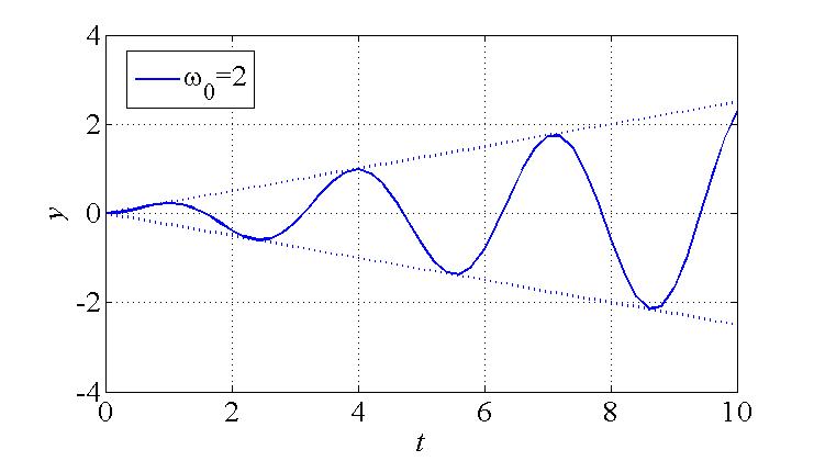
If \({\omega _1} = {\omega _0}\)

\[\left( {{D^2} + \omega _0^2} \right)y = \cos {\omega _0}t \to \left( {{D^2} + \omega _0^2} \right)\widetilde y = {e^{i{\omega _0}t}}\]

\[{\widetilde y_p} = \frac{{t{e^{i{\omega _0}t}}}}{{2i{\omega _0}}} \to {y_p} = \frac{{t\sin {\omega _0}t}}{{2{\omega _0}}}\]

other particular solution: particular solution + part of complementary solution

\[\left( {{D^2} + \omega _0^2} \right)y = \cos {\omega _1}t \to {y_p} = \frac{{\cos {\omega _1}t}}{{\omega _0^2 – \omega _1^2}} – \frac{{\cos {\omega _0}t}}{{\omega _0^2 – \omega _1^2}}\]

\[\mathop {\lim }\limits_{{\omega _1} \to {\omega _0}} \frac{{\cos {\omega _1}t – \cos {\omega _0}t}}{{\omega _0^2 – \omega _1^2}} = \mathop {\lim }\limits_{{\omega _1} \to {\omega _0}} \frac{{ – \sin \left( {{\omega _1}t} \right)t}}{{ – 2{\omega _1}}} = \frac{{t\sin {\omega _0}t}}{{2{\omega _0}}}\]

When the input frequency \({\omega _1}\) approaches the natural frequency \({\omega _0}\), the oscillations obtained by the two methods are the same.

Geometric meaning

\[\frac{{\cos {\omega _1}t – \cos {\omega _0}t}}{{\omega _0^2 – \omega _1^2}} = \frac{{2\sin \frac{{{\omega _0} – {\omega _1}}}{2}t\sin \frac{{{\omega _0} + {\omega _1}}}{2}t}}{{\omega _0^2 – \omega _1^2}} = \frac{{2\sin \frac{{{\omega _0} – {\omega _1}}}{2}t}}{{\omega _0^2 – \omega _1^2}}\sin \frac{{{\omega _0} + {\omega _1}}}{2}t\]

\[{\omega _1} \approx {\omega _0} \to \frac{{\cos {\omega _1}t – \cos {\omega _0}t}}{{\omega _0^2 – \omega _1^2}} \approx \underbrace {\frac{{2\sin \frac{{{\omega _0} – {\omega _1}}}{2}t}}{{\omega _0^2 – \omega _1^2}}}_{{\rm{Amplitute}}}\underbrace {\sin {\omega _0}t}_{{\rm{pure}}\ {\rm{oscillation}}}\]

Damped resonance 

Without input:

\[{x^{\prime\prime}} + 2p{x^{\prime}} + \omega _0^2x =0,\omega _1^2 = \omega _0^2 – {p^2}\]

With input: which \(\omega\) gives the maximal amplitude for the response?

\[{x^{\prime\prime}} + 2p{x^{\prime}} + \omega _0^2x = \cos \omega t \to {\omega _r} = \sqrt {\omega _0^2 – 2{p^2}} \]