Fourier Series

To solve the ODE \({y^{\prime\prime}} + a{y^{\prime}} + by = f\left( t \right)\), in which \(f\left( t \right)\) is often the combination of \({e^t}\), \(\sin t\) and \(\cos t\), then any reasonable \(f\left( t \right)\) which is periodic, can be discontinuous but not terribly discontinuous, can be written as Fourier Series.

\[f\left( t \right) = {c_0} + \sum\limits_{n = 1}^\infty {{a_n}\cos nt + {b_n}\sin nt} \]

Theorem:

\(u\left( t \right),v\left( t \right)\) are functions with period \(2\pi \) on the real number, they are orthogonal (perpendicular) on \(\left[ { – \pi ,\pi } \right]\) if satisfying

\[\int_{ – \pi }^\pi {u\left( t \right)v\left( t \right)} dt = 0\]

\[\left\{ \begin{gathered}
\sin nt \qquad n = 1,2, \cdot \cdot \cdot ,\infty \hfill \\
\cos mt \qquad m = 0,1, \cdot \cdot \cdot ,\infty \hfill \\
\end{gathered} \right.\]

any two distinct ones of those are orthogonal on \(\left[ { – \pi ,\pi } \right]\).

\[\int_{ – \pi }^\pi {\sin nt\cos mt} dt = 0 \qquad \int_{ – \pi }^\pi {{{\sin }^2}nt} dt = \pi \qquad \int_{ – \pi }^\pi {{{\cos }^2}mt} dt = \pi \]

Proof:

We can use trig identities, complex exponential, however the two methods only work on trigonometric functions. The generalized method is to use ODE.

\(\sin nt\) and \(\cos mt\), \(m \ne n\), satisfy

\[{u^{\prime\prime}} + {n^2}u = 0 \to u_n^{\prime\prime} = – {n^2}{u_n}\]

\[{v^{\prime\prime}} + {m^2}v = 0 \to v_m^{\prime\prime} = – {m^2}{v_m}\]

\[\int_{ – \pi }^\pi {u_n^{\prime\prime}{v_m}} dt = \left. {u_n^{\prime}{v_m}} \right|_{ – \pi }^\pi – \int_{ – \pi }^\pi {u_n^{\prime}v_m^{\prime}} dt = – \int_{ – \pi }^\pi {u_n^{\prime}v_m^{\prime}} dt\]

\[\int_{ – \pi }^\pi {u_n^{\prime\prime}{v_m}} dt = – {n^2}\int_{ – \pi }^\pi {{u_n}{v_m}} dt\]

\[\int_{ – \pi }^\pi {v_m^{\prime\prime}{u_n}} dt = – {m^2}\int_{ – \pi }^\pi {{v_m}{u_n}} dt\]

The first equation is symmetric while the second and the third are not symmetric, in fact the \({{u_n}}\) and \({{u_n}}\) are equally important. Thus, the only answer is

\[\int_{ – \pi }^\pi {{u_n}{v_m}} dt = 0,\ m \ne n\]

Calculate the coefficients

\[f\left( t \right) = \cdot \cdot \cdot + {a_k}\cos kt + \cdot \cdot \cdot + {a_n}\cos nt + \cdot \cdot \cdot \]

\[\int_{ – \pi }^\pi {f\left( t \right)} \cos ntdt = \cdot \cdot \cdot + \int_{ – \pi }^\pi {{a_k}\cos kt} \cos ntdt + \cdot \cdot \cdot + \int_{ – \pi }^\pi {{a_n}} {\cos ^2}ntdt + \cdot \cdot \cdot = \int_{ – \pi }^\pi {{a_n}} {\cos ^2}ntdt\]

\[\int_{ – \pi }^\pi {f\left( t \right)} \cos ntdt = {a_n}\pi \to {a_n} = \frac{1}{\pi }\int_{ – \pi }^\pi {f\left( t \right)} \cos ntdt\]

\[{b_n} = \frac{1}{\pi }\int_{ – \pi }^\pi {f\left( t \right)} \sin ntdt\]

\[f\left( t \right) = {c_0} + \cdot \cdot \cdot + {a_n}\cos nt + \cdot \cdot \cdot \]

\[\int_{ – \pi }^\pi {f\left( t \right)} dt = 2\pi {c_0} + \cdot \cdot \cdot + \int_{ – \pi }^\pi {{a_n}\cos nt} dt + \cdot \cdot \cdot = 2\pi {c_0}\]

\[{c_0} = \frac{1}{{2\pi }}\int_{ – \pi }^\pi {f\left( t \right)} dt = \frac{1}{{2\pi }}\int_{ – \pi }^\pi {f\left( t \right)} \cos 0tdt = \frac{{{a_0}}}{2}\]

Example:

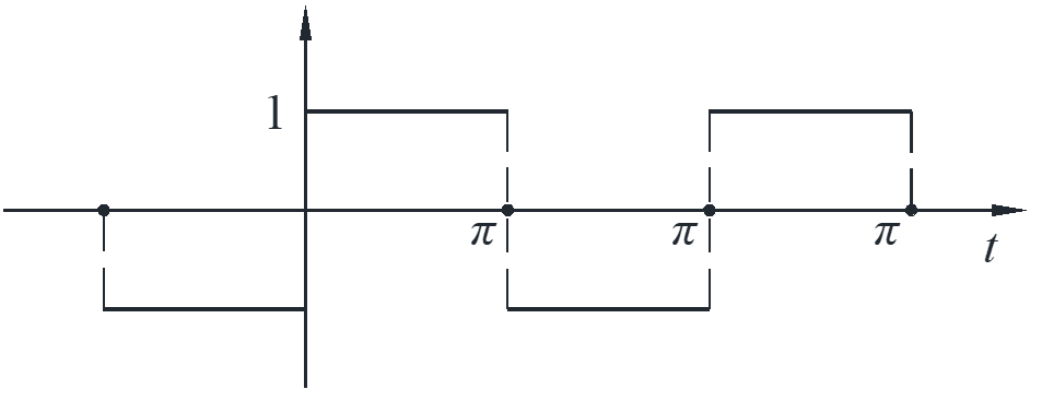
\[{a_n} = 0\]

\[{b_n} = – \frac{1}{\pi }\int_{ – \pi }^0 {\sin nt} dt + \frac{1}{\pi }\int_0^\pi {\sin nt} dt = \frac{{1 – \cos n\pi }}{n} + \frac{{1 – \cos n\pi }}{n} = \frac{2}{n}\left( {1 – \cos n\pi } \right)\]

Extension of  Fourier Series

\[f\left( t \right) = \frac{{{a_0}}}{2} + \sum\limits_{n = 1}^\infty {{a_n}\cos nt + {b_n}\sin nt} \]

\[{a_n} = \frac{1}{\pi }\int_{ – \pi }^\pi {f\left( t \right)} \cos ntdt,{b_n} = \frac{1}{\pi }\int_{ – \pi }^\pi {f\left( t \right)} \sin ntdt\]

Theorem: since there are formulas for \({a_n}\) and \({b_n}\),

\[f\left( t \right) = g\left( t \right) \to F.S.forf\left( t \right) = F.S.forg\left( t \right)\]

1. shorten calculation: use evenness & oddness
2. extend the range of Fourier Series

If \(f\left( t \right)\) is even, \(f\left( { – t} \right) = f\left( t \right)\)

\[f\left( t \right) = \frac{{{a_0}}}{2} + \sum\limits_{n = 1}^\infty {{a_n}\cos nt} ,{b_n} = 0\]

If \(f\left( t \right)\) is odd, \(f\left( { – t} \right) = -f\left( t \right)\)

\[f\left( t \right) = \sum\limits_{n = 1}^\infty {{b_n}\sin nt} ,{a_n} = 0\]

Proof:

\[f\left( { – t} \right) = \frac{{{a_0}}}{2} + \sum\limits_{n = 1}^\infty {{a_n}\cos nt + {b_n}\sin \left( { – nt} \right)} \]

\[f\left( t \right) = \frac{{{a_0}}}{2} + \sum\limits_{n = 1}^\infty {{a_n}\cos nt + {b_n}\sin nt} \]

Thus, \({b_n} = – {b_n}\) for all \(n\), the only answer is \({b_n} = 0\).

Example:

\begin{align*}
{b_n} &= \frac{2}{\pi }\int_0^\pi {t\sin nt} dt = \frac{2}{\pi }\left[ {\left. { – \frac{{t\cos nt}}{n}} \right|_0^\pi – \int_0^\pi {\cos nt} dt} \right] \hfill \\
&= \frac{2}{\pi }\left[ {\left. { – \frac{\pi }{m}{{\left( { – 1} \right)}^n}} \right|_0^\pi \left. { + \frac{{\sin nt}}{n}} \right|_0^\pi } \right] = \frac{2}{m}{\left( { – 1} \right)^{n + 1}} \hfill \\
\end{align*}

\[F.S.forf\left( t \right) = 2\sum\limits_{n = 1}^\infty {\frac{{{{\left( { – 1} \right)}^{n + 1}}}}{m}\sin nt} \]

Theorem:

If \(f\) is continuous at \(t_0\), then \(f\left( t \right) = sum\ of\ its\ F.S.\ at{t_0}\).

If \(f\) is discontinuous at \(t_0\), then \( F.S.\ at{t_0}\) converges to the mid point of the jump.

Extension #1: period \(2L\)

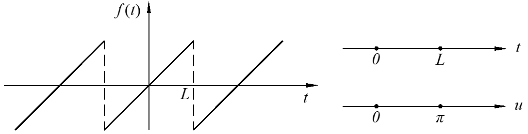
\[f\left( t \right) = \frac{{{a_0}}}{2} + \sum\limits_{n = 1}^\infty {{a_n}\cos n\frac{\pi }{L}t + {b_n}\sin n\frac{\pi }{L}t} \]

\[{a_n} = \frac{1}{L}\int_{ – L}^L {f\left( t \right)} \cos n\frac{\pi }{L}tdt,{b_n} = \frac{1}{L}\int_{ – L}^L {f\left( t \right)} \sin n\frac{\pi }{L}tdt\]

\[t = \frac{L}{\pi }u,u = \frac{\pi }{L}t\]

Extension #2: periodic extension

If \(f\left( t \right)\) is defined on \(\left[ {0,L} \right]\)

Particular solution with Fourier Series

\[{x^{\prime\prime}} + \omega _0^2x = f\left( t \right),f\left( t \right) = \sin \omega t,\cos \omega t \to {x_p} = \frac{{\sin \omega t,\cos \omega t}}{{\omega _0^2 – {\omega ^2}}}\]

\[f\left( t \right) = \frac{{{a_0}}}{2} + \sum\limits_{n = 1}^\infty {{a_n}\cos {\omega _n}t + {b_n}\sin {\omega _n}t} ,{\omega _n} = \frac{{n\pi }}{L}\]

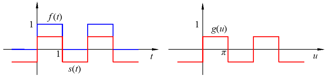
\[f\left( t \right) = s\left( t \right) + \frac{1}{2},s\left( t \right) = \frac{1}{2}g\left( u \right),g\left( u \right) = \frac{4}{\pi }\sum\limits_{odd} {\frac{{\sin nu}}{n}} \]

\[f\left( t \right) = \frac{1}{2} + \frac{1}{2}\frac{4}{\pi }\sum\limits_{odd} {\frac{{\sin n\pi t}}{n}} \]

\[{x_p} = \frac{{{a_0}}}{{\omega _0^2}} + \sum\limits_{n = 1}^\infty {\frac{{{a_n}\cos {\omega _n}t}}{{\omega _0^2 – \omega _n^2}} + \frac{{{b_n}\sin {\omega _n}t}}{{\omega _0^2 – \omega _n^2}}} \]

\[{x_p} = \frac{1}{{2\omega _0^2}} + \frac{2}{\pi }\sum\limits_{odd}^\infty {\frac{{\sin n\pi t}}{{\omega _0^2 – {{\left( {n\pi } \right)}^2}}}} \]

Assume natural frequency \({\omega _0} = 10\), calculate \({x_p}\left( t \right)\)

\begin{align*}
{x_p}\left( t \right) & \approx 0.005 + 0.6\left( {\frac{{\sin \pi t}}{{91}} + \frac{{\sin 3\pi t}}{{45}} – \frac{{\sin 5\pi t}}{{600}}} \right) \hfill \\
&  \approx 0.005 + 0.01\sin \pi t + 0.015\sin 3\pi t – 0.001\sin 5\pi t \hfill \\
\end{align*}

If \({\omega _0} = 9\), near-resonance occurs for frequency \(3\pi \). Frequencies in \(f\left( t \right)\) are hidden, but system picks out resonance with the frequency closest to its natural frequency. Here \({\omega _0} = 10\) and \(n = 3\) is the closest to resonance as the coefficient is largest.

Another method to get the coefficients

Use differential of F.S. term by term and assume solution of form

\[{x_p} = {c_0} + \sum\limits_{n = 1}^\infty {{c_n}\sin n\pi t} \]

substitute into the ODE

\[\omega _0^2{c_0} + \sum\limits_{n = 1}^\infty {{c_n}\left( {\omega _0^2 – {{\left( {n\pi } \right)}^2}} \right)\sin n\pi t} = \frac{1}{2} + \frac{2}{\pi }\sum\limits_{odd} {\frac{{\sin n\pi t}}{n}} \]

by equating coefficients, we can get \(c_n\)

\[{c_0} = \frac{1}{{2\omega _0^2}},{c_n} = \frac{2}{\pi }\frac{1}{{\omega _0^2 – {{\left( {n\pi } \right)}^2}}}\]

Laplace transform

\[\sum\limits_{n = 1}^\infty {{a_n}{x^n}} = A\left( x \right)\]

\[1 \sim \frac{1}{{1 – x}} = 1 + x + {x^2} + {x^3} + \cdot \cdot \cdot ,\frac{1}{{n!}} \sim {e^x} = \sum {\frac{{{x^n}}}{{n!}}} \]

Continuous analog:

\[\int_0^\infty {a\left( x \right){x^t}} dx = A\left( x \right) \to \int_0^\infty {f\left( t \right){e^{ – st}}} dt = F\left( s \right)\]

Laplace transform:

\[L\left( {f\left( t \right)} \right) = F\left( s \right)\]

Linear transform:

\[L\left( {f + g} \right) = L\left( f \right) + L\left( g \right),L\left( {cf} \right) = cL\left( f \right)\]

Commonly used:

\begin{align*}
&1 \mapsto \frac{1}{s},s > 0 \qquad \qquad &\sin at \mapsto \frac{a}{{{s^2} + {a^2}}},s > 0 \\
&{e^{at}} \mapsto \frac{1}{{s – a}} \qquad \qquad  &\cos at \mapsto \frac{s}{{{s^2} + {a^2}}},s > 0 \\
&{e^{at}}f\left( t \right) \mapsto F\left( {s – a} \right),s > a   &{t^n} \mapsto \frac{{n!}}{{{s^{n + 1}}}},s > 0
\end{align*}

Derivation:

\[\int_0^\infty {{e^{ – st}}} dt = \mathop {\lim }\limits_{R \to \infty } \int_0^\infty {{e^{ – st}}} dt = \mathop {\lim }\limits_{R \to \infty } \frac{{{e^{ – sR}} – 1}}{{ – s}} = \frac{1}{s},s > 0\]

\[\int_0^\infty {{e^{at}}f\left( t \right){e^{ – st}}} dt = \int_0^\infty {{e^{at}}f\left( t \right){e^{ – \left( {s – a} \right)t}}} dt = F\left( {s – a} \right),s > a\]

\[{e^{at}} \mapsto \frac{1}{{s – a}},s > a \qquad  {e^{\left( {a + bi} \right)t}} \mapsto \frac{1}{{s – \left( {a + bi} \right)}},s > a\]

\[\cos at = \frac{{{e^{iat}} + {e^{ – iat}}}}{2},L\left( {\cos at} \right) = \frac{1}{2}\left( {\frac{1}{{s – ia}} + \frac{1}{{s + ia}}} \right) = \frac{s}{{{s^2} + {a^2}}},s > 0\]

\[\sin at = \frac{{{e^{iat}} – {e^{ – iat}}}}{2},L\left( {\cos at} \right) = \frac{a}{{{s^2} + {a^2}}},s > 0\]

\[\int_0^\infty {{t^n}{e^{ – st}}} dt = \left. {{t^n}\frac{{{e^{ – st}}}}{{ – s}}} \right|_0^\infty – \int_0^\infty {n{t^{n – 1}}\frac{{{e^{ – st}}}}{{ – s}}} dt = 0 – 0 + \frac{n}{s}\int_0^\infty {{t^{n – 1}}{e^{ – st}}} dt = \frac{n}{s}L\left( {{t^{n – 1}}} \right)\]

\[\mathop {\lim }\limits_{t \to \infty } {t^n}\frac{{{e^{ – st}}}}{{ – s}} = – \frac{1}{s}\mathop {\lim }\limits_{t \to \infty } \frac{{{t^n}}}{{{e^{st}}}} = – \frac{1}{s}\mathop {\lim }\limits_{t \to \infty } \frac{{n{t^{n – 1}}}}{{s{e^{st}}}} = \cdot \cdot \cdot = 0\]

\[L\left( {{t^n}} \right) = \frac{n}{s}L\left( {{t^{n – 1}}} \right) = \cdot \cdot \cdot = \frac{{n\left( {n – 1} \right) \cdot \cdot \cdot 1}}{{{s^n}}}L\left( {{t^0}} \right) = \frac{{n!}}{{{s^{n + 1}}}}\]

inverse Laplace transform

\[{L^{ – 1}}\left( {\frac{1}{{s\left( {s + 3} \right)}}} \right) = {L^{ – 1}}\left( {\frac{{1/3}}{s} + \frac{{ – 1/3}}{{s + 3}}} \right) = \frac{1}{3} – \frac{1}{3}{e^{ – 3t}}\]

Solve ODE with Laplace transform

\[f\left( t \right) \mapsto F\left( s \right) = \int_0^\infty {f\left( t \right){e^{ – st}}} dt,s > 0\]

\begin{align*}
&1 \mapsto \frac{1}{s},s > 0 \qquad \qquad &\sin at \mapsto \frac{a}{{{s^2} + {a^2}}},s > 0 \\
&{e^{at}} \mapsto \frac{1}{{s – a}} \qquad \qquad  &\cos at \mapsto \frac{s}{{{s^2} + {a^2}}},s > 0 \\
&{e^{at}}f\left( t \right) \mapsto F\left( {s – a} \right),s > a   &{t^n} \mapsto \frac{{n!}}{{{s^{n + 1}}}},s > 0
\end{align*}

\(f\left( t \right)\) of “exponential type”

In order to prevent \( f\left( t \right) \) goes up too fast that \(\int_0^\infty {f\left( t \right){e^{ – st}}} dt \approx \infty \), the limitation on  \( f\left( t \right) \)  is

\[\left| {f\left( t \right)} \right| \le c{e^{kt}},c > 0,k > 0\]

\({t^n} \le M{e^t}\) for some \( M \) and all \( t \), as \({t^n}/{e^t}\) starts at zero, ends at zero and is continuous between zero and infinity, it will definitely has the maximum value.

Note #1: \(\frac{1}{t}\) is not an exponential type, because \(\int_0^\infty {\frac{1}{t}} dt \) does not converge.

Note #2: \({e^{{t^2}}}\) is not an exponential type, because no matter how big \( k \) is, \({e^{{t^2}}} > {e^{kt}}\).

Initial value problem IVP

\[{y^{\prime\prime}} + A{y^{\prime}} + by = h\left( t \right),y\left( 0 \right) = {y_0},{y^{\prime}}\left( 0 \right) = y_0^{\prime}\]

Solution: 

Laplace transform on both sides: \[q\left( s \right)\bar Y = p\left( s \right) \to \bar Y = \frac{{p\left( s \right)}}{{q\left( s \right)}}\]

Inverse Laplace transform: \(y\left( t \right)\)

\begin{align*}
L\left( {{f^{\prime}}\left( t \right)} \right) &= \int_0^\infty {{f^{\prime}}\left( t \right){e^{ – st}}} dt = \left. {{e^{ – st}}f\left( t \right)} \right|_0^\infty + \int_0^\infty {s{e^{ – st}}f\left( t \right)} dt\\
& = 0 – f\left( 0 \right) + s\int_0^\infty {{e^{ – st}}f\left( t \right)} dt = sF\left( s \right) – f\left( 0 \right)
\end{align*}

since \({f\left( t \right)}\) is an exponential type,

\[\left| {f\left( t \right)} \right| \le c{e^{kt}} \to \mathop {\lim }\limits_{t \to \infty } \frac{{f\left( t \right)}}{{{e^{st}}}} = 0,\]

\[L\left( {{f^{\prime\prime}}\left( t \right)} \right) = sL\left( {{f^{\prime}}\left( t \right)} \right) – {f^{\prime}}\left( 0 \right) = s\left[ {sF\left( s \right) – f\left( 0 \right)} \right] – {f^{\prime}}\left( 0 \right)\]

\[{f^{\prime}}\left( t \right) \mapsto sF\left( s \right) – f\left( 0 \right),{f^{\prime\prime}}\left( t \right) \mapsto {s^2}F\left( s \right) – sf\left( 0 \right) – {f^{\prime}}\left( 0 \right)\]

Example

\[{y^{\prime\prime}} – y = {e^{ – t}},y\left( 0 \right) = 1,{y^{\prime}}\left( 0 \right) = 0\]

\[{s^2}\bar Y – s \cdot 1 – 0 – \bar Y = \frac{1}{s}\]

\[\bar Y = \frac{{{s^2} + s + 1}}{{{{\left( {s + 1} \right)}^2}\left( {s – 1} \right)}} = \frac{{ – 1/2}}{{{{\left( {s + 1} \right)}^2}}} + \frac{{1/4}}{{s + 1}} + \frac{{3/4}}{{s – 1}}\]

\[y\left( t \right) = \underbrace { – \frac{1}{2}t{e^{ – t}}}_{{y_p}} + \underbrace {\frac{1}{4}{e^{ – t}} + \frac{3}{4}{e^t}}_{{y_c}}\]

Convolution

\[f\left( t \right) * g\left( t \right) = \int_0^t {f\left( u \right)} g\left( {u – t} \right)du\]

Proof:

\[F\left( s \right) = \int_0^\infty {{e^{ – st}}f\left( t \right)} dt,G\left( s \right) = \int_0^\infty {{e^{ – st}}g\left( t \right)} dt\]

\[F\left( s \right)G\left( s \right) = \int_0^\infty {{e^{ – st}}\left( {f\left( t \right) * g\left( t \right)} \right)} dt \to f\left( t \right) * g\left( t \right) \mapsto F\left( s \right)G\left( s \right)\]

\begin{align*}
F\left( s \right)G\left( s \right) &= \int_0^\infty {{e^{ – su}}f\left( u \right)} du \cdot \int_0^\infty {{e^{ – sv}}g\left( v \right)} dv = \int_0^\infty {\int_0^\infty {{e^{ – s\left( {u + v} \right)}}f\left( u \right)g\left( v \right)} } dudv\\
&= \int_0^\infty {\int_0^t {{e^{ – st}}f\left( u \right)g\left( {t – u} \right)} } dudt = \int_0^\infty {{e^{ – st}}\left( {\int_0^t {f\left( u \right)g\left( {t – u} \right)du} } \right)} dt\\
&= \int_0^\infty {{e^{ – st}}\left( {f\left( t \right) * g\left( t \right)} \right)} dt
\end{align*}

It should be noted about the limits of the

\[dudt = \frac{{\partial \left( {u,v} \right)}}{{\partial \left( {u,t} \right)}}dudt,J = \frac{{\partial \left( {u,v} \right)}}{{\partial \left( {u,t} \right)}} = \left| {\begin{array}{*{20}{c}}
{\frac{{\partial u}}{{\partial u}}}&{\frac{{\partial u}}{{\partial t}}}\\
{\frac{{\partial v}}{{\partial u}}}&{\frac{{\partial v}}{{\partial t}}}
\end{array}} \right| = 1\]

Example:

\begin{align*}
{t^2} * t &= \int_0^t {{u^2}\left( {t – u} \right)du} = \frac{{{t^4}}}{{12}}\\
&= {L^{ – 1}}\left( {\frac{{2!}}{{{s^3}}} \cdot \frac{1}{{{s^2}}}} \right) = {L^{ – 1}}\left( {\frac{2}{{{s^5}}}} \right) = 2 \cdot \frac{{{t^4}}}{{4!}} = \frac{{{t^4}}}{{12}}
\end{align*}

\[f\left( t \right) * 1 = \int_0^t {f\left( t \right) \cdot 1du} = \int_0^t {f\left( t \right)du} \]

Application:

the dumping rate of radioactive waste is \(f\left( t \right)\) in years, and the left amount due to decaying is \({A_0}{e^{ – kt}}\) assuming \(k\) is fixed, \(A_0\) is the initial amount of waste and \(t\) is the amount of time left. By the time \(t\), how much waste is left?

In the time period \(\left[ {{u_i},{u_{i + 1}}} \right]\), the amount of left is

\[f\left( {{u_i}} \right) \cdot \Delta u \cdot {e^{ – k\left( {t – {u_i}} \right)}} = \int_0^t {f\left( u \right){e^{ – k\left( {t – u} \right)}}du} = f\left( t \right) * {e^{ – kt}}\]

Dealing with discontinuity with Laplace transform

Jump discontinuity

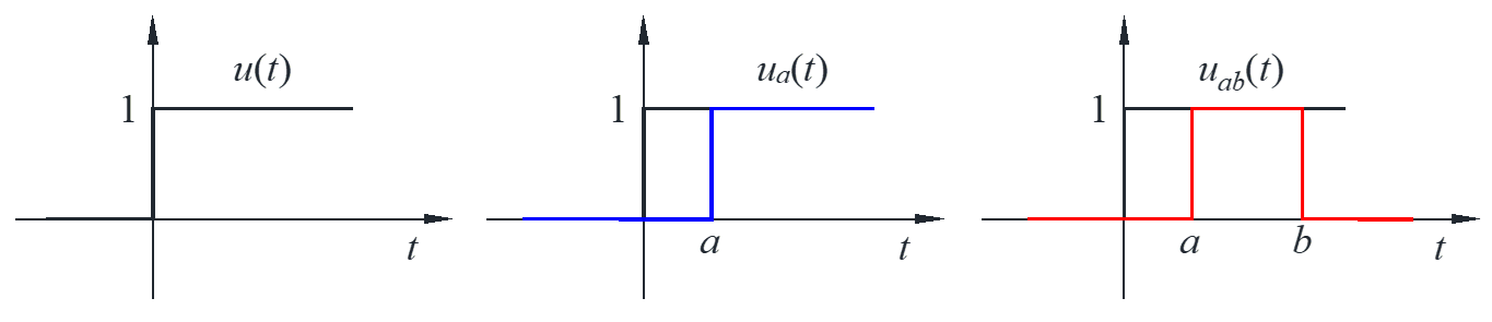
\(u\left( t \right)\) is the unit step and \(u\left( 0 \right)\) is not defined shown as the black line. Translate \(u\left( t \right)\) to the right shown as the blue line, we get

\[{u_a}\left( t \right) = u\left( {t – a} \right)\]

Thus, the “unit box” shown as the red line is then

\[{u_{ab}}\left( t \right) = {u_a}\left( t \right) – {u_b}\left( t \right) = u\left( {t – a} \right) – u\left( {t – b} \right)\]

To make the inverse Laplace transform unique, we need to multiply a unit step with the \(f\left( t \right)\), as we do not care about the formula of  \(f\left( t \right)\) when  \(t<0\).

\[L\left( {f\left( t \right)} \right) = F\left( s \right),{L^{ – 1}}\left( {F\left( s \right)} \right) = u\left( t \right)f\left( y \right)\]

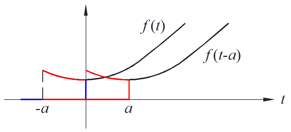
We want a formula \(L\left( {f\left( {t – a} \right)} \right)\) in terms of \(L\left( {f\left( {t} \right)} \right)\), however this formula does not exist because we do not need the line \(t<0\) for \(L\left( {f\left( {t} \right)} \right)\), but we need the part \(-a<t<0\) to get \(L\left( {f\left( {t – a} \right)} \right)\), as figured.

\begin{align*}
u\left( {t – a} \right)f\left( {t – a} \right) &\mapsto {e^{ – as}}F\left( s \right) \qquad  &{\rm{the \ right \ formula}}\\
u\left( {t – a} \right)f\left( t \right) &\mapsto {e^{ – as}}L\left( {f\left( {t + a} \right)} \right) \qquad  &{\rm{t – axis \ translation \ formula}}
\end{align*}

Proof:

\begin{align*}
\int_0^\infty {{e^{ – st}}u\left( {t – a} \right)f\left( {t – a} \right)dt} &= \int_{ – a}^\infty {{e^{ – s\left( {{t_1} + a} \right)}}u\left( {{t_1}} \right)f\left( {{t_1}} \right)d{t_1}} = {e^{ – sa}}\int_{ – a}^\infty {{e^{ – s{t_1}}}u\left( {{t_1}} \right)f\left( {{t_1}} \right)d{t_1}} \\
&= {e^{ – sa}}\int_0^\infty {{e^{ – s{t_1}}}u\left( {{t_1}} \right)f\left( {{t_1}} \right)d{t_1}} = {e^{ – sa}}F\left( s \right)
\end{align*}

We get \(u\left( {t – a} \right)f\left( {t – a} \right) \mapsto {e^{ – as}}F\left( s \right)\) by replace \(t \to t + a\) to get the right side, so

\[u\left( {t – a} \right)f\left( t \right) = u\left( {t – a} \right)f\left( {t – a + a} \right) \mapsto {e^{ – as}}L\left( {f\left( {t + a} \right)} \right)\]

Example:

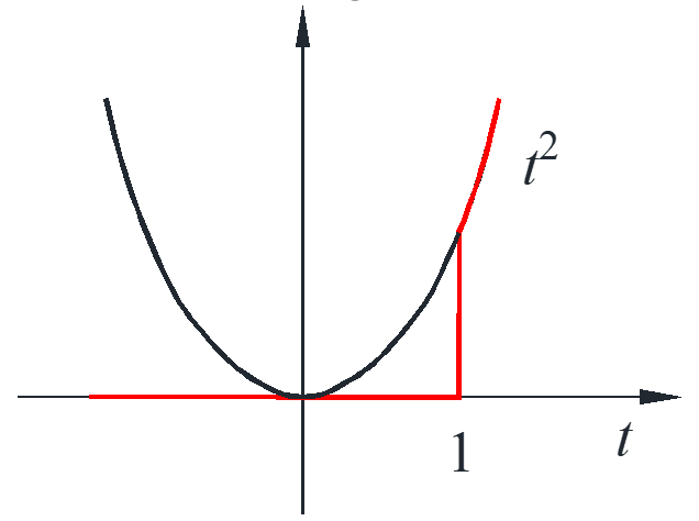
\begin{align*}
u\left( {t – 1} \right){t^2} \mapsto {e^{ – s}}L\left( {{{\left( {t + 1} \right)}^2}} \right) &= {e^{ – s}}L\left( {{t^2} + 2t + 1} \right)\\
&= {e^{ – s}}\left( {\frac{2}{{{s^3}}} + \frac{2}{{{s^2}}} + \frac{1}{s}} \right)
\end{align*}

There are three terms in the result, as we can see from the curve, there are two parts and one discontinuous point \(t=1\), as indicate by the result \({e^{ – s}}\).

\[{L^{ – 1}}\left( {\frac{{1 + {e^{ – \pi s}}}}{{{s^2} + 1}}} \right) = {L^{ – 1}}\left( {\frac{1}{{{s^2} + 1}} + \frac{{{e^{ – \pi s}}}}{{{s^2} + 1}}} \right) = u\left( t \right)\sin \left( t \right) + u\left( {t – \pi } \right)\sin \left( {t – \pi } \right) = f\left( t \right)\]

\[f\left( t \right) = \left\{ \begin{align*}
\sin t \qquad \qquad \qquad \qquad &0 \le t \le \pi \\
\sin t + \sin \left( {t – \pi } \right) = 0 \qquad &t \ge \pi
\end{align*} \right.\]

It should be noted that \({L^{ – 1}}\left( {\frac{1}{{{s^2} + 1}}} \right) = u\left( t \right)\sin \left( t \right)\), in which the \(u\left( t \right)\) can not be omitted because there is an exponential type in this example, which means the function has been translated along the x-axis.

Dirac delta function

impulse of  \(f\left( t \right)\) over the time period \(\left[ {a,b} \right]\) is defined as

\[\int_a^b {f\left( t \right)dt} \]

\[\frac{1}{h}{u_{0h}}\left( t \right) = \frac{1}{h}\left[ {u\left( t \right) – u\left( {t – h} \right)} \right] \mapsto \frac{1}{h}\left[ {\frac{1}{s} – \frac{{{e^{ – hs}}}}{s}} \right]\]

\[\mathop {\lim }\limits_{h \to 0} \frac{{1 – {e^{ – hs}}}}{{hs}} = \mathop {\lim }\limits_{u \to 0} \frac{{1 – {e^{ – u}}}}{u} = \frac{{{e^{ – u}}}}{1} = 1\]

Dirac delta function:

\[\delta \left( t \right) \mapsto 1 \qquad \int_0^\infty {\delta \left( t \right)dt} = 1\]

\[u\left( t \right)f\left( t \right) * \delta \left( t \right) \mapsto F\left( s \right) \cdot 1,{u^{\prime}}\left( t \right) = \delta \left( t \right)\]

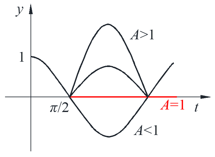
Example: kick a ball with impulse \(A\) at \(t=\pi /2\)

\[{y^{\prime\prime}} + y = A\delta \left( {t – \frac{\pi }{2}} \right),y\left( 0 \right) = 1,{y^{\prime}}\left( 0 \right) = 0\]

\[{s^2}\bar Y – s + \bar Y = A{e^{ – \pi /2}} \cdot 1 \to \bar Y = \frac{s}{{{s^2} + 1}} + \frac{{A{e^{ – \pi /2}}}}{{{s^2} + 1}}\]

\[y = u\left( t \right)\cos t + u\left( {t – \pi /2} \right) \cdot A\sin \left( {t – \pi /2} \right)\]

\[y = \left\{ \begin{align*}
\cos t \qquad \qquad \qquad \qquad & 0 \le t \le \pi /2\\
\cos t + A\sin \left( {t – \pi /2} \right) = \left( {1 – A} \right)\cos t \qquad & t \ge \pi /2
\end{align*} \right.\]

Note that the solution to this ODE is continuous, the curve is described as follow whit different values of \(A\), which means after the time \(t=\pi /2\) with the impulse \(A\), the motion of the ball would stop or keep going or go backward depending on the magnitude of \(A\).

Solution to ODE

\[{y^{\prime\prime}} + a{y^{\prime}} + by = f\left( t \right),y\left( 0 \right) = 0,{y^{\prime}}\left( 0 \right) = 0\]

\[{s^2}\bar Y + as\bar Y + b\bar Y = F\left( s \right) \to \bar Y = \frac{{F\left( s \right)}}{{{s^2} + as + b}}\]

\[y\left( t \right) = f\left( t \right) * w\left( t \right) = \int_0^u {f\left( u \right)w\left( {t – u} \right)du} \]

\[{\rm{weight \ function \ of \ system}} \quad w\left( t \right) \mapsto W\left( s \right) = \frac{1}{{{s^2} + as + b}} \quad {\rm{transfer \ function}}\]

What is \(w\left( t \right)\), really? Assume a ball kicked by impulse at \(t=0\) with the ODE

\[{y^{\prime\prime}} + a{y^{\prime}} + by = \delta \left( t \right),y\left( 0 \right) = 0,{y^{\prime}}\left( 0 \right) = 0\]

\[\bar Y = \frac{1}{{{s^2} + as + b}} \to y\left( t \right) = w\left( t \right)\]