Euler equation:
\[\left\{ \begin{align}
& {{x}_{n+1}}={{x}_{n}}+h \\
& {{y}_{n+1}}={{y}_{n}}+{{A}_{n}}h \\
\end{align} \right.\]
\[\left\{ \begin{align}
& h=\text{step}\text{size} \\
& {{A}_{n}}=f\left( {{x}_{n}},{{y}_{n}} \right) \\
\end{align} \right.\]
Error of solution
error = exact solution – approximate solution
Method 1: smaller step
Euler first-order: \(e\sim {{c}_{1}}h\), proportional to step size
Method 2: find a better slop \({{A}_{n}}\)
Heun’s method = improved Euler method = modified Euler method = RK2
\[\left\{ \begin{align}
& {{x}_{n+1}}={{x}_{n}}+h \\
& {{y}_{n+1}}={{y}_{n}}+h\left( \frac{{{A}_{n}}+{{B}_{n}}}{2} \right) \\
\end{align} \right.\]
in which, \({{B}_{n}}=f\left( {{x}_{n+1}},{{y}_{n+1}} \right)\)
Second-order method: \(e \sim c{h^2}\)
Method 3: RK4
Standard method – accurate, used in computer programs
Rung-Kutta method
\[\frac{{{A}_{n}}+2{{B}_{n}}+2{{C}_{n}}+{{D}_{n}}}{6}\]
Pitfalls
#1 Find in assignments
#2 Singularity
Ex. \({{y}^{\prime}}={{y}^{2}}\)
Solus: \(y=\frac{1}{c-x}\) with singularity at \(x=c\), \(y(2)=\infty \)
First-order linear ODE
\[a(x){{y}^{\prime}}+b(x)y=c(x)\]
when \(c\left( x \right) = 0\), the equation is homogeneous.
Standard linear form: the coefficient of \({{y}^{\prime}}\) equals to 1.
\[{{y}^{\prime}}+p(x)y=q(x)\]
Models: Temp-conc model (Temperature-concentration model), Decay model, Bank account, Motion
Newton cooling law: \(\frac{dT}{dt}=k\left( {{T}_{e}}-T \right)\)
t = time, T = temperature, \(k > 0\) is the conductivity
Diffusion model: \(\frac{dC}{dt}=k\left( {{C}_{e}}-C \right)\)
C = salt concentration inside
Derivation of solution method
\[{{y}^{\prime}}+p(x)y=q(x)\]
\[u{{y}^{\prime}}+puy=qu\]
\[{{\left( uy \right)}^{\prime}}=qu\]
\[{{u}^{\prime}}=pu\to \frac{{{u}^{\prime}}}{u}=p\to \ln u=p\to u={{e}^{\int{pdx}}}\]
\(u(x)\) is defined as integration factor
Method:
- standard linear form
- calculate integration factor \({{e}^{\int{pdx}}}\)
- multiply both sides by \({{e}^{\int{pdx}}}\)
- integrate
Example 1:
\[\left( 1+\cos x \right){{y}^{\prime}}-\left( \sin x \right)y=2x\]
- \({{y}^{\prime}}-\frac{\sin x}{1+\cos x}y=\frac{2x}{1+\cos x}\)
- I.F. \({{e}^{\int{\frac{\sin x}{1+\cos x}dx}}}={{e}^{\ln \left( 1+\cos x \right)}}=1+\cos x\)
- \(\left( 1+\cos x \right){{y}^{\prime}}-\left( \sin x \right)y=2x\)
- \({{\left[ \left( 1+\cos x \right)y \right]}^{\prime}}=2x\to \left( 1+\cos x \right)y={{x}^{2}}+c\to y=\frac{{{x}^{2}}+c}{1+\cos x}\)
Example 2: linear with constant k
Temp: \(\frac{dT}{dt}+kT=k{{T}_{e}}\)
- I.F. \({{e}^{kt}}\)
- \({{\left( {{e}^{kt}}T \right)}^{\prime}}=k{{T}_{e}}{{e}^{kt}}\)
- \({{e}^{kt}}T=\int{k{{T}_{e}}\left( t \right){{e}^{kt}}}dt+c\)
- \(T={{e}^{-kt}}\int{k{{T}_{e}}\left( t \right){{e}^{kt}}}dt+c{{e}^{-kt}}\)
\({{e}^{-kt}}\int{k{{T}_{e}}\left( t \right){{e}^{kt}}}dt\) is steady state solution, and \(c{{e}^{-kt}}\) is transient solution because \(k>0,t\to \infty ,c{{e}^{-kt}}\to 0\).
Changing variables
scaling: \({{x}_{1}}=\frac{x}{a},{{y}_{1}}=\frac{y}{b}\)
Aims:
- change units
- make variables dimensionless
- reduce the number of constants, or simplify constants
Newton cooling law: \(\frac{dT}{dt}=k\left( {{M}^{4}}-{{T}^{4}} \right)\)
T=internal temperature, M=constant external temperature
\[{{T}_{1}}=\frac{T}{M}\to T={{T}_{1}}M\]
\[M\frac{dT}{dt}=k{{M}^{4}}\left( 1-T_{1}^{4} \right)\to \frac{dT}{dt}=k{{M}^{3}}\left( 1-T_{1}^{4} \right)\]
Direct substitution and indirect substitution
Bernoulli equation: \[{{y}^{\prime}}=p(x)y+q(x){{y}^{n}}\left( n\ne 0 \right)\]
\[\frac{{{y}^{\prime}}}{{{y}^{n}}}=p(x)\frac{1}{{{y}^{n-1}}}+q(x)\]
\[v=\frac{1}{{{y}^{n-1}}}={{y}^{1-n}}\to {{v}^{\prime}}=\left( 1-n \right){{y}^{-n}}{{y}^{\prime}}\]
\[\frac{{{v}^{\prime}}}{1-n}=p(x)v+q(x)\]
we can get linear equation then.
Example 1:
\[{{y}^{\prime}}=\frac{y}{x}+{{y}^{2}}\Rightarrow y=\frac{2x}{{{x}^{2}}+c}\]
Homogeneous ODE
Invariant under the operation zoom:
\[{{y}^{\prime}}=F\left( y/x \right)\]
Example: \({{y}^{\prime}}=\frac{{{x}^{2}}y}{{{x}^{3}}+{{y}^{3}}}=\frac{y/x}{1+{{(y/x)}^{3}}}\)
Example 1
The light try to track a boat on the sea and the boat travels at a angle of 45° with the light, as figured below, what is the travel path of the boat, assuming the initial point is \(\left( {x,y} \right)\).
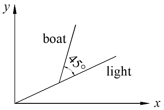
\[{{y}^{\prime}}=\tan \left( \alpha +{{45}^{\circ }} \right)=\frac{\tan \alpha +\tan {{45}^{\circ }}}{1-\tan \alpha \tan {{45}^{\circ }}}\]
\[{{y}^{\prime}}=\frac{y/x+1}{1-y/x}=\frac{y+x}{x-y}\]
\[z=y/x\to {{y}^{\prime}}={{z}^{\prime}}x+z\]
\[{{z}^{\prime}}x+z=\frac{z+1}{1-z}\]
\[x\frac{dz}{dx}=\frac{z+1}{1-z}-z=\frac{1+{{z}^{2}}}{1-z}\]
\[\frac{1+{{z}^{2}}}{1-z}dz=\frac{1}{x}dx\]
\[\left( \frac{1}{1+{{z}^{2}}}-\frac{z}{1+{{z}^{2}}} \right)dz=\frac{1}{x}dx\]
\[{{\tan }^{-1}}z-\frac{1}{2}\ln \left( 1+{{z}^{2}} \right)=\ln x+c\]
\[{{\tan }^{-1}}\left( \frac{y}{x} \right)=\ln x+\ln \sqrt{1+\frac{{{y}^{2}}}{{{x}^{2}}}}+c=\ln \sqrt{{{x}^{2}}+{{y}^{2}}}+c\]
\[\theta =\ln r+c\to r={{c}_{1}}{{e}^{\theta }}\]
Exponential spiral: \(r=c{{e}^{\theta }}\)
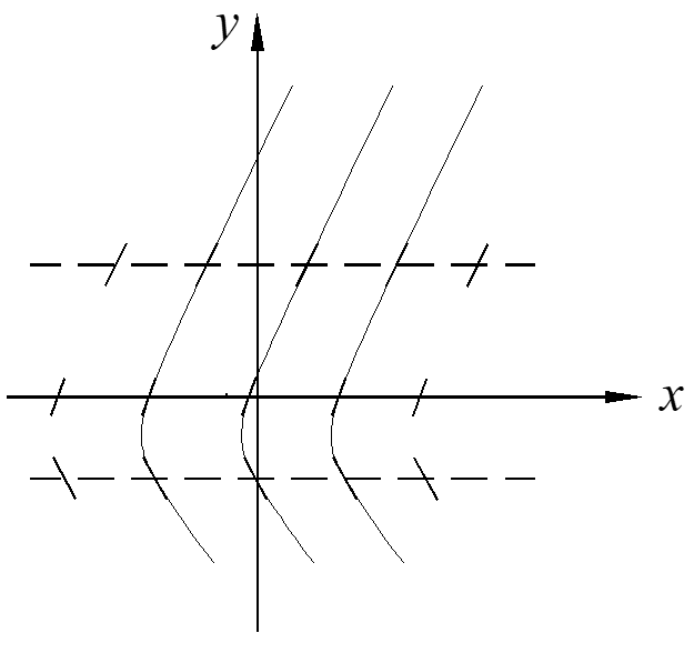
Autonomous First-order ODE
No independent variables on the right
\[\frac{dy}{dt}=f\left( y \right)\]
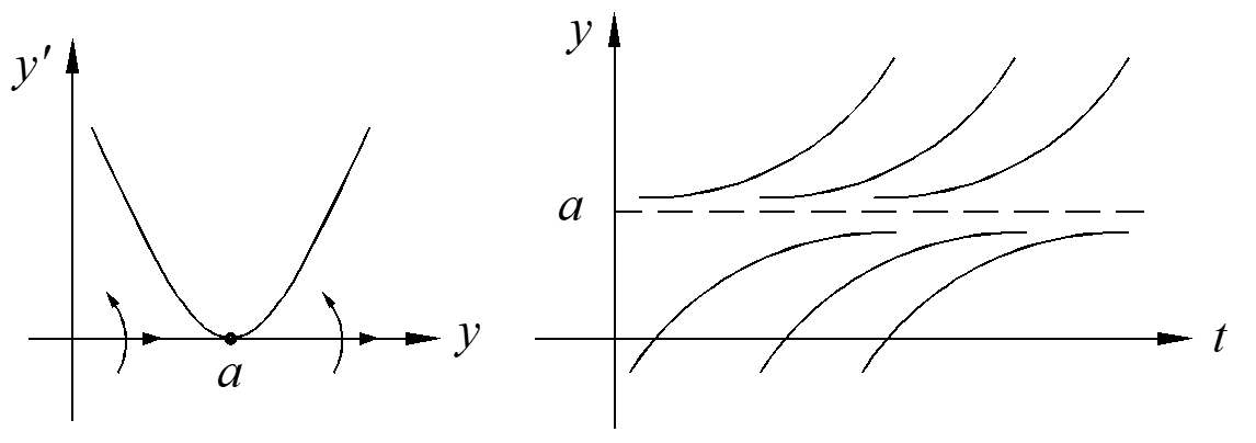
It is not easy to get the solution, but we can get qualitative information about the solution with direction field. For any t, \(f\left( y \right) = \) constant, which means the slopes are the same. Thus, the curves of solutions can be translated along the x-axis.
The critical point: \({{y}^{\prime}}=f\left( {{y}_{0}} \right)=0\) or \(y={{y}_{0}}\) is a solution.
Proof: \(\frac{d{{y}_{0}}}{dt}=0=f\left( {{y}_{0}} \right)\), both sides of the equation equal to zero.
Method to know the qualitative information of the solution:
- find the critical points
- graph \(f\left( y \right) \), if \(f\left( y \right) > 0 \), the solution increases, or decreases
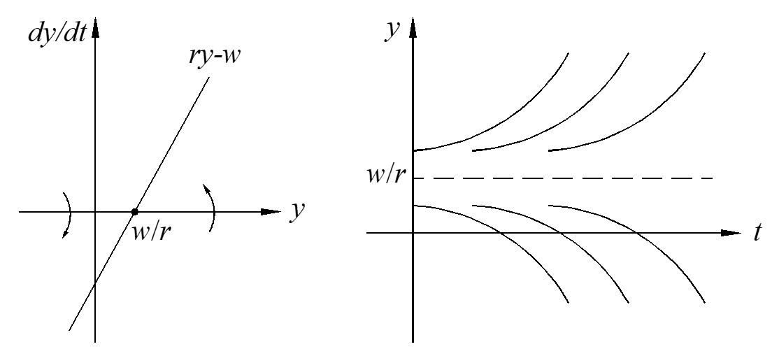
Example: y is the money in account, r is the continuous interest, w is the rate of embezzlement with certain amount.
\[\frac{dy}{dt}=ry-w\]
critical point: \[y-w=0\to y=\frac{w}{r}\]
Logistic Equation
Population behavior: \(y\left( t \right)\), k = growth rate. If k = constant, this is simple growth. If \(k\ne \)constant, this is Logistic growth. Normally k declines as y increases, and we choose the simplest one \(k=a-by\), then the population behavior is:
\[\frac{dy}{dt}=ay-b{{y}^{2}}\]
Obviously, we can get the solution of this equation by separating variables and though partial integration. Here we only look at the characteristic of the solution. The critical points can be calculated as
\[ay-b{{y}^{2}}=0\to y=0,y=\frac{a}{b}\]
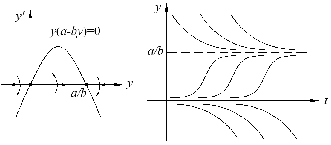
The critical point \(y=\frac{a}{b}\) is a stable critical point because the solutions goes close, the point \(y=0\) is an unstable critical point because the solutions goes away.
What is there is only one critical point? The critical point is stable on one side and unstable on the other side, which can be called simi-stable critical point, as shown below.
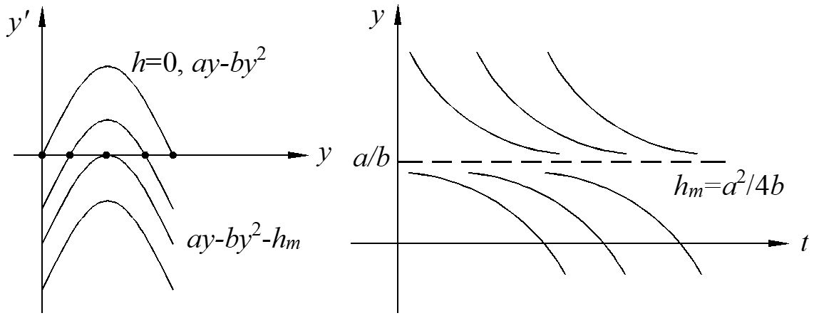
Logistic Equal with Harvesting
Assuming the harvest at constant time rate is h. This model is very useful for animal or plant raising.
\[\frac{dy}{dt}=ay-b{{y}^{2}}-h\]
The maximum time rate is \({{h}_{m}}=\frac{{{a}^{2}}}{4b}\), which is the only critical point of the solution.
Complex number
\[{{i}^{2}}=-1\]
\[z=a+bi,\overline{z}=a-bi\]
Polar representation
\[a+bi=r\cos \theta +ir\sin \theta =r{{e}^{i\theta }}\]
Euler definition: \({{e}^{i\theta }}=\cos \theta +i\sin \theta \)
Exponential function:
- exponential law: \({{e}^{i{{\theta }_{1}}}}{{e}^{i{{\theta }_{2}}}}={{e}^{i({{\theta }_{1}}+{{\theta }_{2}})}}\)
- initial value: \[{{e}^{i*0}}=1\]
- infinite series: \(\frac{d}{dt}{{e}^{it}}={{e}^{it}}\)
Proof 1:
\[\begin{align}
& {{e}^{i{{\theta }_{1}}}}{{e}^{i{{\theta }_{2}}}}=(\cos {{\theta }_{1}}+i\sin {{\theta }_{1}})(\cos {{\theta }_{2}}+i\sin {{\theta }_{2}})=(\cos {{\theta }_{1}}\cos {{\theta }_{2}}-\sin {{\theta }_{1}}\sin {{\theta }_{2}})+i(\cos {{\theta }_{1}}\sin {{\theta }_{2}}+\cos {{\theta }_{2}}\sin {{\theta }_{1}}) \\
& =\cos ({{\theta }_{1}}+{{\theta }_{2}})+i\sin ({{\theta }_{1}}+{{\theta }_{2}})={{e}^{i({{\theta }_{1}}+{{\theta }_{2}})}} \\
\end{align}\]
Proof 2:
\[{{e}^{i*0}}=\cos 0+i\sin 0=1\]
Proof 3:
\[\frac{d}{dt}{{e}^{it}}=\frac{d}{dt}(\cos t+i\sin t)=-\sin t+i\cos t=i(\cos t+i\sin t)={{e}^{it}}\]
Advantage of polar representation: good for multiplication
Example:
\[\int{{{e}^{-x}}\cos xdx}=\operatorname{Re}\left( \int{{{e}^{(-1+i)x}}} \right)=\frac{1}{2}{{e}^{-x}}\left( -\cos x+\sin x \right)\]
\[\int{{{e}^{(-1+i)x}}}=\frac{{{e}^{(-1+i)x}}}{-1+i}=\frac{1}{-1+i}{{e}^{-x}}\left( \cos x+i\sin x \right)=\frac{-1-i}{2}{{e}^{-x}}\left( \cos x+i\sin x \right)\]
\(\sqrt[n]{1}\) has n answers as complex numbers. For example, \(\sqrt[5]{1}\) can be expressed with a circle with radius equals to 1 and the circle is divided with five lines equally, as shown below.
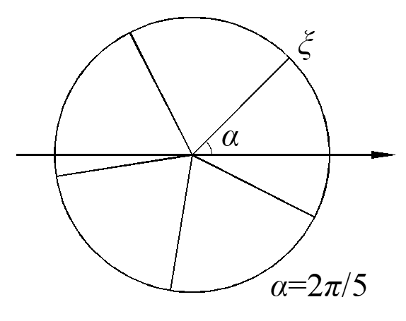
\[\xi ={{e}^{i\frac{2}{5}\pi }}\to {{\xi }^{5}}={{e}^{i\frac{2}{5}\pi \cdot 5}}={{e}^{2\pi i}}=1\]
First-order differential equation with complex numbers
\[{{y}^{\prime}}+ky=q\left( t \right)\]
Solution:
\[y={{e}^{-kt}}\int{q\left( t \right){{e}^{kt}}dt}+c{{e}^{-kt}}\]
The first part \({{e}^{-kt}}\int{q\left( t \right){{e}^{kt}}dt}\) is steady-state solution, also called long-term solution, the second part \(c{{e}^{-kt}}\) is transient solution. We usually choose the simplest answer as steady-state solution, usually c=0. If k>0, the solution is steady solution, the solution goes close to the steady-state value, otherwise, the solution is transient.
\[{{y}^{\prime}}+ky=k{{q}_{e}}\left( t \right),{{q}_{e}}\left( t \right)=\cos wt\]
w = angular frequency = number of complete oscillation
complexified equation:
\[{\widetilde y^{\prime}} + k\widetilde y = k{e^{iwt}}\]
complex solution: \[\widetilde y = {y_1} + i{y_2}\]
\[y = {\rm{real}}{\kern 1pt} {\kern 1pt} {\kern 1pt} {\rm{part}}{\kern 1pt} {\kern 1pt} {\kern 1pt} {\rm{of}}{\kern 1pt} {\kern 1pt} \widetilde y\]
\[{\left( {\widetilde y{e^{ – kt}}} \right)^{\prime}} = k{e^{(k + wi)t}} \to \widetilde y{e^{ – kt}} = \frac{k}{{k + iw}}{e^{(k + wi)t}}\]
\[\widetilde y = \frac{{k\left( {k – iw} \right)}}{{{k^2} + {w^2}}}{e^{iwt}} = \frac{1}{{1 + i\frac{w}{k}}}{e^{iwt}}\]
Method 1: Go polar
Reminder: \(\alpha \) is a complex number, then
\[\frac{1}{\alpha } \cdot \alpha = 1 \to \arg \left( {\frac{1}{\alpha }} \right) + \arg \left( \alpha \right) = \arg \left( 1 \right) = 0 \to \arg \left( {\frac{1}{\alpha }} \right) – \arg \left( \alpha \right)\]
\[\frac{1}{\alpha } \cdot \alpha = 1 \to \left| {\frac{1}{\alpha }} \right| = \frac{1}{{\left| \alpha \right|}}\]
Polar form:
\[\frac{1}{{1 + i\left( {w/k} \right)}} = A{e^{ – i\phi }} = \frac{1}{{\sqrt {1 + {{\left( {w/k} \right)}^2}} }}{e^{ – i\phi }}\]
\[\arg \left( {1 + i\frac{w}{k}} \right) \to \phi = {\tan ^{ – 1}}\left( {w/k} \right)\]
So, the solution of the ODE , which is the real part of the complex solution, is
\[\widetilde y = A{e^{iwt – i\phi }} = \frac{1}{{\sqrt {1 + {{\left( {w/k} \right)}^2}} }}{e^{i\left( {wt – \phi } \right)}} \to {y_1} = \frac{1}{{\sqrt {1 + {{\left( {w/k} \right)}^2}} }}\cos \left( {wt – \phi } \right)\]
in which, \(A\) is the amplitude and \(\phi \) is the phase lag. If the conductivity \(k\) increases, the amplitude \(A\) also increases, which is consistent with our common sense.
Method 2: Go Cartesian
\[\widetilde y = \frac{1}{{1 + i\left( {w/k} \right)}}{e^{iwt}} = \frac{{1 – i\left( {w/k} \right)}}{{1 + {{\left( {w/k} \right)}^2}}}\left( {\cos wt + i\sin wt} \right)\]
\[\begin{array}{l}
{y_1} = \frac{1}{{1 + {{\left( {w/k} \right)}^2}}}\left( {\cos wt + \left( {w/k} \right)\sin wt} \right) = \frac{1}{{1 + {{\left( {w/k} \right)}^2}}}\sqrt {1 + {{\left( {w/k} \right)}^2}} \cos \left( {wt – \phi } \right)\\
{\kern 1pt} {\kern 1pt} {\kern 1pt} {\kern 1pt} {\kern 1pt} {\kern 1pt} {\kern 1pt} {\kern 1pt} {\kern 1pt} {\kern 1pt} {\kern 1pt} {\kern 1pt} = \frac{1}{{\sqrt {1 + {{\left( {w/k} \right)}^2}} }}\cos \left( {wt – \phi } \right)
\end{array}\]
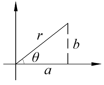
The following equation is used in the derivation, which is very important and we can just remember it with the triangle as figured above.
\[a\cos \theta + b\sin \theta = c\cos \left( {\theta – \phi } \right),{\kern 1pt} {\kern 1pt} c = \sqrt {{a^2} + {b^2}} ,{\kern 1pt} {\kern 1pt} {\kern 1pt} \phi = {\tan ^{ – 1}}\left( {b/a} \right)\]
Proof of this equation:
Method 1: high school method, write all from the right side and compare with the left side.
Method 2: 18.08 proof
\[ < a,b > \cdot < \cos \theta ,\sin \theta > = \left| { < a,b > } \right| \cdot 1 \cdot \cos \left( {\theta – \phi } \right)\]
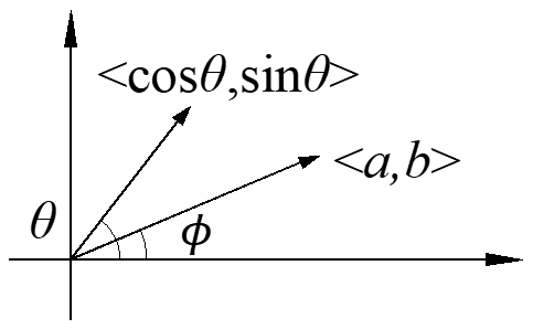
Definition: \(\overrightarrow a \cdot \overrightarrow b = \sum\limits_{i = 1}^n {{a_i}{b_i}} = {a_1}{b_1} + {a_2}{b_2} + \cdot \cdot \cdot + {a_n}{b_n} = \left| a \right|\left| b \right|\cos \theta \)
Method 3: 18.03 proof
\[\left( {a – bi} \right)\left( {\cos \theta + i\sin \theta } \right) = \sqrt {{a^2} + {b^2}} {e^{ – i\phi }} \cdot {e^{i\theta }} = \sqrt {{a^2} + {b^2}} {e^{i\left( {\theta – \phi } \right)}}\]
Take real parts of both sides:
\[a\cos \theta + b\sin \theta = \sqrt {{a^2} + {b^2}} \cos \left( {\theta – \phi } \right)\]
Summary: basic linear ODE
\[{y^{\prime}} + ky = k{q_e}\left( t \right),{\kern 1pt} {\kern 1pt} {\kern 1pt} {\kern 1pt} {\kern 1pt} {\kern 1pt} k > 0\]
\[{y^{\prime}} + ky = q\left( t \right)\]
\[{y^{\prime}} + p\left( t \right)y = q\left( t \right)\]
Mixing example
\(x\left( t \right)\) = amount of salt in tank at time t, \({C_e}\) = concentration of incoming salt, V is the volume of the tank, r = rate of salt inflow = rate of salt outflow. Then, the variation of salt in tank equals to the amount of salt inflow minus the amount of salt outflow expressed by equation:
\[\frac{{dx}}{{dt}} = r{C_e} – r\frac{x}{V}\]
Standard form: \[\frac{{dC}}{{dt}} + \frac{r}{V}C = \frac{r}{V}{C_e}\]
How dose the tank concentration \(C\left( t \right)\) follows the inflow salt concentration ({C_e}\left( t \right)\)? If the volume of the tank V is very small, then the tank concentration \(C\left( t \right)\) is very close to \({C_e}\left( t \right)\), so the the amplitude \(A \approx 1\) and \(\phi \approx 0\).
For the second kind of linear ODE, if \(k < 0\), none of the terminology of transient, steady-state input response applies. However, \(k < 0\) is used in economy, biology etc. expressed in the following equation.
\[\frac{{dy}}{{dt}} – ay = q\left( t \right),a > 0\]