Calculation of transverse shear stiffness
Definition
The effective transverse shear stiffness of the section of a shear flexible beam is defined in Abaqus as
\[{\overline K _{\alpha 3}} = f_p^\alpha {K_{\alpha 3}}\]
where \({\overline K _{\alpha 3}}\) is the section shear stiffness in the \(\alpha \)-direction; \({K_{\alpha 3}}\) is the actual shear stiffness of the section having units of force; and \(\alpha = 1,{\kern 1pt} {\kern 1pt} {\kern 1pt} 2\) are the local directions of the cross-section. \(f_p^\alpha \) is a dimensionless factor used to prevent the shear stiffness from becoming too large in slender beam elements and is always included in the calculation of transverse shear stiffness defined as
\[f_p^\alpha = \frac{1}{{1 + \xi \cdot SCF\frac{{{l^2}A}}{{12{I_{\alpha \alpha }}}}}}\]
where l is the length of the element, A is the cross-sectional area, \({{I_{\alpha \alpha }}}\) is the inertia in the \(\alpha \)-direction, SCF is the slenderness compensation factor (with a default value of 0.25), and \(\xi \) is a constant of value 1.0 for first-order elements and 10-4 for second-order elements.
For meshed cross-sections the above expressions change to
\[\overline K _{\alpha \beta }^{ts} = {f_p}K_{\alpha \beta }^{ts}\]
\[{f_p} = \frac{1}{{1 + \xi \cdot SCF\frac{{{l^2}\left( {EA} \right)}}{{12{{\left( {EI} \right)}_{\alpha v}}}}}}\]
\[{\left( {EI} \right)_{\alpha v}} = \frac{{{{\left( {EI} \right)}_{11}} + {{\left( {EI} \right)}_{22}} + {{\left( {EI} \right)}_{12}}}}{2}\]
You can define the \({K_{\alpha 3}}\) or \(K_{\alpha \beta }^{ts}\) as described below. If you do not specify them, they are defined by
\({K_{\alpha 3}} = kGA\) or \(K_{\alpha \beta }^{ts} = k{\left( {GA} \right)_{\alpha \beta }}\)
where G is the elastic shear modulus or moduli of the beam section. Temperature and field variable dependencies of G are not taken into account when calculating \({K_{\alpha 3}}\) and \(K_{\alpha \beta }^{ts}\). The shear factor k (Cowper, 1966) is adopted in ABAQUS referring to Abaqus Analysis User’s Guide.
Keywords edition
First (and only) line:
- Value of the shear stiffness of the section in the first direction, \(K_{11}^{ts}\).
- Value of the shear stiffness of the section in the second direction, \(K_{22}^{ts}\).
- Value of the coupling term in the shear stiffness of the section, \(K_{12}^{ts}\).
If either value \(K_{11}^{ts}\) or \(K_{22}^{ts}\) is omitted or given as zero, the nonzero value will be used for both.
- Value of the \(K_{23}\) shear stiffness of the section.
- Value of the \(K_{13}\) shear stiffness of the section.
-
Value of the slenderness compensation factor or the label SCF. If this field is left blank, a default value of 0.25 is assumed. If the label SCF is specified, the values of the shear stiffness specified by the user will be ignored. They and the slenderness compensation factor will be calculated from the elastic material definition with the beam section.
If either value \({K_{\alpha 3}}\) is omitted or given as zero, the nonzero value will be used for both when the label SCF is not used.
Notes in 29.3.3 Choosing a beam element :
You can also define the slenderness compensation factor. The default value for the slenderness compensation factor is 0.25. If a slenderness compensation factor value is provided, you must also provide the values of the shear stiffness \({K_{\alpha 3}}\).
In the case of first-order elements, you may define the slenderness compensation factor by including the label SCF. Abaqus will then use a slenderness compensation factor of \(SCF = \frac{{kGA}}{{EA}}\) , and any values of \({K_{\alpha 3}}\) that you specify are ignored. Instead, the \({K_{\alpha 3}}\) values are calculated from the elastic material definition.
The transverse shear stiffness is not relevant to Euler-Bernoulli beam elements for which the transverse shear constraints are satisfied exactly.
Verification examples
The model for verification is the same as that in Beam elements in ABAUQS. Both the first-order and second-order elements are adopted in this example.
First-order element B31
The default value of SCF for first-order elements is defined as \(SCF = \frac{{kGA}}{{EA}}\) and in this example default SCF=0.2. The dimensionless factor \(f_p^\alpha \) with different SCF values are adopted for comparison. The stiffness factor in the following list is a scale of actual shear stiffness \({K_{\alpha 3}}\) and the relative values of section shear stiffness \({\overline K _{\alpha 3}}\) are also given.
| SCF | dimensionless \(f_p^\alpha \) | stiffness factor | relative value of \({\overline K _{\alpha 3}}\) |
| 0.20 | 0.9954 | 1 | 0.9954 |
| 0.0001 | 1.0000 | 1 | 1.0000 |
| 0.25 | 0.9944 | 1 | 0.9944 |
| 0.25 | 0.9944 | 0.643 | 0.6394 |
| 0.25 | 0.9944 | 10.7 | 10.6401 |
| 0.25 | 0.9944 | 100 | 99.4398 |
| 0.25 | 0.9944 | 1000 | 994.3976 |
| 25 | 0.6396 | 1 | 0.6396 |
| 2500 | 0.0174 | 1 | 0.0174 |
| 250000 | 0.0002 | 1 | 0.0002 |
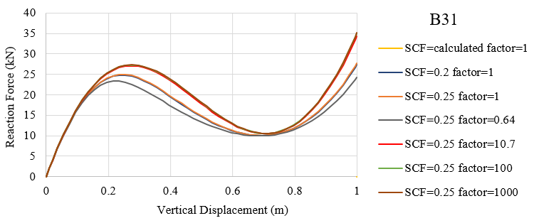
The force-displacement curves with SCF=(0.0001, 0.2, calculated in abaqus, 0.25) and stiffness factor=1 are very close to each other with the relative values of \({\overline K _{\alpha 3}}\) approach to 1.0. Also, curves with SCF=0.25, stiffness factor=(10.7, 100, 1000) accord well with each other with the relative values of \({\overline K _{\alpha 3}}\) greater than 10.0 and vary each other. The obvious differences between curves with SCF=0.25, stiffness factor=(1, 0.64, 10.7) are observed in the above figure and the resistance of frame enhances with higher transverse shear stiffness.
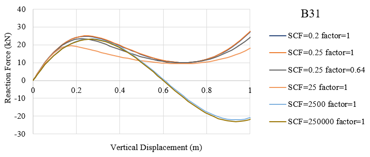
With the increase in SCF value (0.25, 25, 2500, 250000) and a constant stiffness factor 1.0, the relative value of \({\overline K _{\alpha 3}}\) decreases and the curves lower. The difference between SCF values (2500, 250000) is slight and conclusion can be made that when the the relative value of \({\overline K _{\alpha 3}}\) is lower than 0.02, the displacements of structures are similar with different SCF values.
It is noted that the relative values of \({\overline K _{\alpha 3}}\) with (SCF, stiffness)=(0.25, 0.643) and (25, 1) are very close while the curves differ. The reason for this is unclear for me.
Second-order element B32
The default value of SCF for second-order elements is 0.25 and different SCF values same as above are adopted for comparison. Similar procedures are utilized and similar conclusions can be drawn.
| SCF | dimensionless \(f_p^\alpha \) | stiffness factor | relative value of \({\overline K _{\alpha 3}}\) |
| 0.0001 | 1.0000 | 1 | 1.0000 |
| 0.25 | 1.0000 | 1 | 1.0000 |
| 0.25 | 1.0000 | 0.64 | 0.6400 |
| 0.25 | 1.0000 | 10 | 10.0000 |
| 0.25 | 1.0000 | 100 | 99.9999 |
| 0.25 | 1.0000 | 1000 | 999.9994 |
| 25 | 0.9999 | 1 | 0.9999 |
| 2500 | 0.9944 | 1 | 0.9944 |
| 250000 | 0.6396 | 1 | 0.6396 |

The force-displacement curves with SCF=(0.000001, 0.25, calculated in abaqus) and stiffness factor=1 are very close to each other with the relative values of \({\overline K _{\alpha 3}}\) equal to 1.0. Also, curves with SCF=0.25, stiffness factor=(10, 100, 1000) accord well with each other with the relative values of \({\overline K _{\alpha 3}}\) greater than 10.0 and vary each other. The obvious differences between curves with SCF=0.25, stiffness factor=(1, 0.64, 10) are observed in the above figure. The resistance of frame enhances with higher transverse shear stiffness and the enhancement is limited.
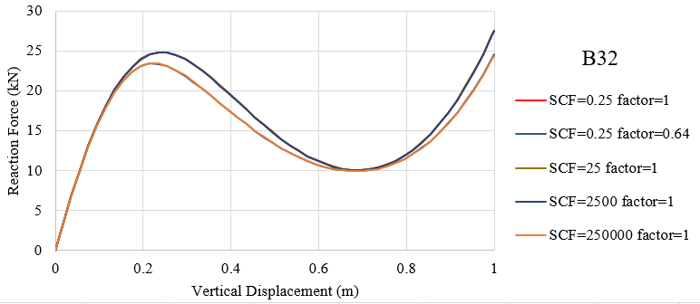
The relative values of \({\overline K _{\alpha 3}}\) with SCF=(0.25, 25, 2500) and a constant stiffness factor 1.0 are almost the same and the curves of them are also close to each other. The relative values of \({\overline K _{\alpha 3}}\) with (SCF, stiffness)=((0.25, 0.64) and (250000, 1) are very close to each other and the curves accord well meeting the regulation of similar values. Conclusion can be drawn that the force-displacement curve is in direct proportion to the relative value of effective shear stiffness.
Notes:
- The explanations in Keywords *TRANSVERSE SHEAR STIFFNESS and in 29.3.3 Choosing a beam element are not the same. It is found that both the SCF and shear stiffness you defined will be used to calculate the effective transverse shear stiffness.
- However, I do not know why the force-displacement curves are different with the same relative values of effective shear stiffness for first-order element B31.
-
Since the \(\xi \) is a constant of value 1.0 for first-order elements and 10-4 for second-order elements, smaller element length are require to ensure \(f_p^\alpha \) close to 1 when you define the shear stiffness in Abaqus. In short, the \(f_p^\alpha \) is always included and fine mesh is preferred for both B31 and B32 elements. With B32 elements, you can have the same results with relatively coarse mesh compared with B31 element.
1 comments On Transverse shear stiffness of beam in ABAQUS
I was recommended this web site by my cousin. I am not sure whether this post is written by him as nobody else know such detailed about my trouble. You are wonderful! Thanks!