Limit theorem

Chebyshev’s inequality

$$\begin{align} {\sigma ^2} &= \int {{{\left( {x – \mu } \right)}^2}{f_X}\left( x \right)dx} \\ &\ge \int_{ – \infty }^{u – c} {{{\left( {x – \mu } \right)}^2}{f_X}\left( x \right)dx} + \int_{u + c}^\infty {{{\left( {x – \mu } \right)}^2}{f_X}\left( x \right)dx} \\ &\ge {c^2}\int_{ – \infty }^{u – c} {{f_X}\left( x \right)dx} {\rm{ + }}{c^2}\int_{u + c}^\infty {{f_X}\left( x \right)dx} \\ &={c^2}{\rm{P}}\left( {\left| {X – \mu } \right| \ge c} \right) \end{align}$$

$${\rm{P}}\left( {\left| {X – \mu } \right| \ge c} \right) \le \frac{{{\sigma ^2}}}{{{c^2}}} \to {\rm{P}}\left( {\left| {X – \mu } \right| \ge k\sigma } \right) \le \frac{1}{{{k^2}}}$$

Convergence

$${M_n} = \frac{{{X_1} + \cdots + {X_n}}}{n}$$

$$\begin{align} {\rm{E}}\left[ {{M_n}} \right] &= \frac{{{\rm{E}}\left[ {{X_1}} \right] + \cdots + {\rm{E}}\left[ {{X_n}} \right]}}{n} = \frac{{n\mu }}{n} = \mu \\ {\mathop{\rm var}} \left( {{M_n}} \right) &= \frac{{{{\left( {{X_1} – \mu } \right)}^2} + \cdots + {{\left( {{X_n} – \mu } \right)}^2}}}{{{n^2}}} = \frac{{n{\sigma ^2}}}{{{n^2}}} = \frac{{{\sigma ^2}}}{n} \to 0\\ {\rm{P}}\left( {\left| {{M_n} – \mu } \right| \ge \varepsilon } \right) &\le \frac{{{\mathop{\rm var}} \left( {{M_n}} \right)}}{{{\varepsilon ^2}}} = \frac{{{\sigma ^2}}}{{n{\varepsilon ^2}}} \to 0 \end{align}$$

Example

Bernoulli process ${\sigma _x} = p\left( {1 – p} \right) = \frac{1}{4}$

95% confidence of error smaller than 1% ${\rm{P}}\left( {\left| {{M_n} – \mu } \right| \ge 0.01} \right) \le 0.05$

$$\begin{align} {\rm{P}}\left( {\left| {{M_n} – \mu } \right| \ge 0.01} \right) &\le \frac{{\sigma _{{M_n}}^2}}{{{{0.01}^2}}} = \frac{{\sigma _x^2}}{{{{0.01}^2}n}}\\ &\le \frac{1}{{4n{{\left( {0.01} \right)}^2}}} \le 0.05 \end{align}$$

Scaling of $M_n$

$$\begin{align} {S_n} = {X_1} + \cdots + {X_n} &\to {\mathop{\rm var}} \left( {{S_n}} \right) = n{\sigma ^2}\\ {M_n} = \frac{{{S_n}}}{n} &\to {\mathop{\rm var}} \left( {{M_n}} \right) = \frac{{{\sigma ^2}}}{n}\\ \frac{{{S_n}}}{{\sqrt n }} &\to {\mathop{\rm var}} \left( {\frac{{{S_n}}}{{\sqrt n }}} \right) = \frac{{{\mathop{\rm var}} \left( {{S_n}} \right)}}{n} = {\sigma ^2} \end{align}$$

Central limit theorem

Standardized ${S_n} = {X_1} + \cdots + {X_n}$

$${Z_n} = \frac{{{S_n} – {\rm{E}}\left[ {{S_n}} \right]}}{{{\sigma _{{S_n}}}}} = \frac{{{S_n} – n{\rm{E}}\left[ X \right]}}{{\sqrt n \sigma }} \sim N\left( {0,1} \right)$$

$${\rm{P}}\left( {{Z_n} \le c} \right) \to {\rm{P}}\left( {Z \le c} \right) = \Phi \left( c \right)$$

CDF of ${Z_n}$ converges to normal CDF, not about convergence of PDF or PMF

Example: 

$n = 36,p = 0.5$, find ${\rm{P}}\left( {{S_n} \le 21} \right)$

Exact answer:

$$\sum\limits_{k = 0}^{21} {\left( {\begin{array}{*{20}{c}} {36}\\ k \end{array}} \right)} {\left( {\frac{1}{2}} \right)^{36}} = 0.8785$$

Method 1: Central limit theorem

$${Z_n} = \frac{{{S_n} – n{\rm{E}}\left[ X \right]}}{{\sqrt n \sigma }} = \frac{{{S_n} – np}}{{\sqrt {np\left( {1 – p} \right)} }}$$

$$\begin{align} {\rm{E}}\left[ {{S_n}} \right] &= np = 36 \cdot 0.5 = 18\\ \sigma _{{S_n}}^2 &= np\left( {1 – p} \right) = 9\\ {\rm{P}}\left( {{S_n} \le 21} \right) &\approx {\rm{P}}\left( {\frac{{{S_n} – 18}}{3} \le \frac{{21 – 18}}{3}} \right) = {\rm{P}}\left( {{Z_n} \le 1} \right) = 0.843 \end{align}$$

Method 2: 1/2 correction for binomial approximation

$$\begin{align} {\rm{P}}\left( {{S_n} \le 21} \right) &= {\rm{P}}\left( {{S_n} < 22} \right)\ \ \ {S_n}{\rm{\ is\ an\ integer}}\\ {\rm{P}}\left( {{S_n} \le 21.5} \right) &\approx {\rm{P}}\left( {{Z_n} \le \frac{{21.5 – 18}}{3}} \right) = {\rm{P}}\left( {{Z_n} \le 1.17} \right) = 0.879 \end{align}$$

The solution is closer to the exact answer.

De Moivre-Laplace CLT

When 1/2 correction is used, CLT can also approximate the binomial pmf, not just the binomial CDF.

$$\begin{align} {\rm{P}}\left( {{S_n} = 19} \right) &= {\rm{P}}\left( {18.5 \le {S_n} \le 19.5} \right) \approx {\rm{P}}\left( {0.17 \le {Z_n} \le 0.5} \right)\\ &= {\rm{P}}\left( {{Z_n} \le 0.5} \right) – {\rm{P}}\left( {{Z_n} \le 0.17} \right) = 0.124 \end{align}$$

Exact answer: ${\rm{P}}\left( {{S_n} = 19} \right) = \left( {\begin{array}{*{20}{c}} {36}\\ {19} \end{array}} \right){\left( {\frac{1}{2}} \right)^{36}} = 0.125$

Poisson arrivals during unit interval equals: sum of $n$ (independent) Poisson arrivals during $n$ intervals of length $1/n$. $X = {X_1} + \cdots + {X_n}$, ${\rm{E}}\left[ X \right] = 1$. Fix $p$ of $X_i$, when $n \to \infty$, the mean and variance are changing, so CLT cannot be applied here. For Binomial$\left( {n,p} \right)$:

$$\begin{align} p \ {\rm{fixed}},n &\to \infty : \ {\rm{normal}}\\ np \ {\rm{fixed}},n &\to \infty : \ {\rm{Poisson}} \end{align}$$

Bayesian statistical inference

Types of Inference models/approaches

$$X=aS+W$$

#1. Model building: know “signal” $S$, observe $X$, infer $a$

#2. Inferring unknown variables: know $a$, observe $X$, infer $S$

#3. Hypothesis testing: unknown takes one of few possible values, aim at small probability of incorrect decision

#4. Estimation: aim at a small estimation error

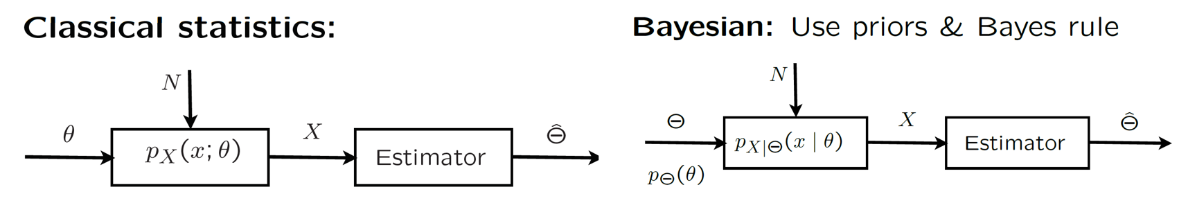
$\theta$ is an unknown parameter and the difference between classical statistics and Bayesian is that $\theta$ is constant in classical statistics, but a random variable in Bayesian.

$$\begin{align} {p_{\Theta \left| X \right.}}\left( {\theta \left| x \right.} \right) = \frac{{{p_\Theta }\left( \theta \right){f_{\Theta \left| X \right.}}\left( {\theta \left| x \right.} \right)}}{{{f_X}\left( x \right)}}& \qquad {\rm{Hypothesis \ testing}}\\ {f_{\Theta \left| X \right.}}\left( {\theta \left| x \right.} \right) = \frac{{{f_\Theta }\left( \theta \right){f_{\Theta \left| X \right.}}\left( {\theta \left| x \right.} \right)}}{{{f_X}\left( x \right)}}& \qquad {\rm{Estimation}} \end{align}$$

Maximum a posteriori probability (MAP): choose a single value that gives a maximum probability, often used in hypothesis testing, but may be misleading when look into the conditional expectation.

Least mean squares estimation (LMS): find $c$ to minimize ${\rm{E}}\left[ {{{\left( {\Theta – c} \right)}^2}} \right]$, in which $c = {\rm{E}}\left[ \Theta \right]$, then the optimal mean squared error is ${\mathop{\rm var}} \left( \Theta \right) = {\rm{E}}\left[ {{{\left( {\Theta – {\rm{E}}\left[ \Theta \right]} \right)}^2}} \right]$, summarized as

$${\rm{minimize \ E}}\left[ {{{\left( {\Theta – c} \right)}^2}} \right] \to c = {\rm{E}}\left[ \Theta \right] \to {\mathop{\rm var}} \left( \Theta \right) = {\rm{E}}\left[ {{{\left( {\Theta – {\rm{E}}\left[ \Theta \right]} \right)}^2}} \right]$$

$$\begin{align} {\rm{E}}\left[ {{{\left( {\Theta – c} \right)}^2}} \right] &= {\rm{E}}\left[ {{\Theta ^2}} \right] – 2c{\rm{E}}\left[ \Theta \right] + {c^2}\\ \frac{d}{{dc}}{\rm{E}}\left[ {{{\left( {\Theta – c} \right)}^2}} \right] &= – 2{\rm{E}}\left[ \Theta \right] + 2c = 0 \end{align}$$

LMS estimation of two random variables

$$\begin{align} {\rm{minimize \ E}}\left[ {{{\left( {\Theta – c} \right)}^2}\left| {X = x} \right.} \right] &\to c = {\rm{E}}\left[ {\Theta \left| {X = x} \right.} \right]\\ {\mathop{\rm var}} \left( {\Theta \left| {X = x} \right.} \right) = {\rm{E}}\left[ {{{\left( {\Theta – {\rm{E}}\left[ {\Theta \left| {X = x} \right.} \right]} \right)}^2}\left| {X = x} \right.} \right] &\le {\rm{E}}\left[ {{{\left( {\Theta – g\left( x \right)} \right)}^2}\left| {X = x} \right.} \right]\\ {\rm{E}}\left[ {{{\left( {\Theta – {\rm{E}}\left[ {\Theta \left| X \right.} \right]} \right)}^2}\left| X \right.} \right] &\le {\rm{E}}\left[ {{{\left( {\Theta – g\left( x \right)} \right)}^2}\left| X \right.} \right]\\ {\rm{E}}\left[ {{{\left( {\Theta – {\rm{E}}\left[ \Theta \right]} \right)}^2}} \right] &\le {\rm{E}}\left[ {{{\left( {\Theta – g\left( x \right)} \right)}^2}} \right] \end{align}$$

LMS estimation with several measurements: ${\rm{E}}\left[ {\Theta \left| {{X_1}, \cdots ,{X_n}} \right.} \right]$, is hard to compute and involves multi-dimensional integrals, etc.

Estimator: $\widehat \Theta = {\rm{E}}\left[ {\Theta \left| X \right.} \right]$, with estimation error $\widetilde \Theta = \widehat \Theta – \Theta$

$$\begin{array}{l} {\rm{E}}\left[ {\widetilde \Theta \left| X \right.} \right] = {\rm{E}}\left[ {\widehat \Theta – \Theta \left| X \right.} \right] = {\rm{E}}\left[ {\widehat \Theta \left| X \right.} \right] – {\rm{E}}\left[ {\Theta \left| X \right.} \right] = \widehat \Theta – \widehat \Theta = 0\\ {\rm{E}}\left[ {\widetilde \Theta h\left( x \right)\left| X \right.} \right] = h\left( x \right){\rm{E}}\left[ {\widetilde \Theta \left| X \right.} \right] = 0 \to {\rm{E}}\left[ {\widetilde \Theta h\left( x \right)} \right] = 0\\ {\mathop{\rm cov}} \left( {\widetilde \Theta ,\widehat \Theta } \right) = {\rm{E}}\left[ {\left( {\widetilde \Theta – {\rm{E}}\left[ {\widetilde \Theta } \right]} \right) \cdot \left( {\widehat \Theta – {\rm{E}}\left[ {\widehat \Theta } \right]} \right)} \right] = {\rm{E}}\left[ {\widetilde \Theta \cdot \left( {\widehat \Theta – \Theta } \right)} \right] = 0\\ \widetilde \Theta = \widehat \Theta – \Theta \to {\mathop{\rm var}} \left( \Theta \right) = {\mathop{\rm var}} \left( {\widehat \Theta } \right) + {\mathop{\rm var}} \left( {\widetilde \Theta } \right) \end{array}$$

Linear LMS

Consider estimator of $\Theta$ of the form $\widehat \Theta = aX + b$ and minimize ${\rm{E}}\left[ {{{\left( {\Theta – aX – b} \right)}^2}} \right]$

$${\widehat \Theta _L} = {\rm{E}}\left[ \Theta \right] + \frac{{{\mathop{\rm cov}} \left( {X,\Theta } \right)}}{{{\mathop{\rm var}} \left( X \right)}}\left( {X – {\rm{E}}\left[ X \right]} \right)$$

$${\rm{E}}\left[ {{{\left( {{{\widehat \Theta }_L} – \Theta } \right)}^2}} \right] = \left( {1 – {\rho ^2}} \right)\sigma _\Theta ^2$$

Consider estimators of the form $\widehat \Theta = {a_1}{X_1} + \cdots + {a_n}{X_n} + b$ and minimize ${\rm{E}}\left[ {{{\left( {{a_1}{X_1} + \cdots + {a_n}{X_n} + b – \Theta } \right)}^2}} \right]$. Set derivatives to zero and linear system in $b$ and the $a_i$, only means, variances, covariances matter.

Cleanest linear LMS example

${X_i} = \Theta + {W_i}$, $\Theta ,{W_1}, \cdots ,{W_n}$ are independent, $\Theta \sim \mu ,\sigma _0^2$ and ${W_i} \sim 0,\sigma _i^2$, then

$${\widehat \Theta _L} = \frac{{\mu /\sigma _0^2 + \sum\limits_{i = 1}^n {{X_i}/\sigma _i^2} }}{{\sum\limits_{i = 1}^n {1/\sigma _i^2} }}$$

Classical statistical inference

Problem type

#1: hypothesis testing ${H_0}:\theta = 1/2 \ {\rm{versus}} \ {H_1}:\theta = 3/4$

#2: composite hypotheses ${H_0}:\theta = 1/2 \ {\rm{versus}} \ {H_1}:\theta \ne 1/2$

#3: estimation, design an estimator $\widehat \Theta$ to keep estimation error $\widehat \Theta – \theta$ small

Maximum likelihood estimation: pick $\theta$ that makes data most likely

$${\widehat \theta _{MAP}} = \arg \mathop {\max }\limits_\theta {p_\Theta }\left( {x;\theta } \right)$$

Example: $\mathop {\max }\limits_\theta \mathop \Pi \limits_{i = 1}^n \theta {e^{ – \theta {x_i}}}$

$$\begin{align} \mathop {\max }\limits_\theta \mathop \Pi \limits_{i = 1}^n \theta {e^{ – \theta {x_i}}} &\to \mathop {\max }\limits_\theta \left( {n\log \theta – \theta \sum\limits_{i = 1}^n {{x_i}} } \right)\\ \frac{n}{\theta } – \sum\limits_{i = 1}^n {{x_i}} = 0 &\to {\widehat \theta _{ML}} = \frac{n}{{{x_1} + \cdots + {x_n}}} \end{align}$$

desirable properties of estimators

(1) unbiased: ${\rm{E}}\left[ {{{\widehat \Theta }_n}} \right] = \theta$

(2) consistent: ${\widehat \Theta _n} \to \theta$ in probability

(3) small mean squared error (MSE): ${\rm{E}}\left[ {{{\left( {\widehat \Theta – \theta } \right)}^2}} \right] = {\mathop{\rm var}} \left( {\widehat \Theta – \theta } \right) + \left( {{\rm{E}}\left[ {\widehat \Theta – \theta } \right]} \right) = {\mathop{\rm var}} \left( {\widehat \Theta } \right) + {\left( {{\rm{biased}}} \right)^2}$

Confidence intervals (CIs)

random interval $\left[ {\widehat \Theta _n^ – ,\widehat \Theta _n^ + } \right]$ with an $1 – \alpha$ confidence interval

$${\rm{P}}\left( {\widehat \Theta _n^ – \le \theta \le \widehat \Theta _n^ + } \right) \ge 1 – \alpha$$

CI in estimation of the mean ${\widehat \Theta _n} = \left( {{X_1} + \cdots + {X_n}} \right)/n$

$$\Phi \left( {1.96} \right) = 1 – 0.05/2$$

$${\rm{P}}\left( {\frac{{\left| {{{\widehat \Theta }_n} – \theta } \right|}}{{\sigma /\sqrt n }} \le 1.96} \right) \approx 0.95$$

$${\rm{P}}\left( {{{\widehat \Theta }_n} – \frac{{1.96\sigma }}{{\sqrt n }} \le \theta \le {{\widehat \Theta }_n} + \frac{{1.96\sigma }}{{\sqrt n }}} \right) \approx 0.95$$

more generally

$$\Phi \left( z \right) = 1 – \alpha /2 \to {\rm{P}}\left( {{{\widehat \Theta }_n} – \frac{{z\sigma }}{{\sqrt n }} \le \theta \le {{\widehat \Theta }_n} + \frac{{z\sigma }}{{\sqrt n }}} \right) \approx 1 – \alpha$$

Since the $\sigma$ is unknown, then we should estimate the value of $\sigma$

option 1: upper bound on $\sigma$, for example Bernoulli $\sigma = \sqrt {p\left( {1 – p} \right)} \le 1/2$

option 2: ad hoc estimate of $\sigma$, for example Bernoulli$\theta$, $\widehat \sigma = \sqrt {\widehat \Theta \left( {1 – \widehat \Theta } \right)}$

option 3: generic estimation of the variance

$$\begin{array}{l} {\sigma ^2} = {\rm{E}}\left[ {{{\left( {{X_i} – \theta } \right)}^2}} \right]\\ \widehat \sigma _n^2 = \frac{1}{n}\sum\limits_{i = 1}^n {{{({X_i} – \theta )}^2}} \to {\sigma ^2}\\ \widehat S_n^2 = \frac{1}{{n – 1}}\sum\limits_{i = 1}^n {{{({X_i} – {{\widehat \Theta }_n})}^2}} \to {\sigma ^2} \end{array}$$