ODE system
\[\left\{ \begin{array}{l}
{x^{\prime}} = f\left( {x,y,t} \right)\\
{y^{\prime}} = g\left( {x,y,t} \right)
\end{array} \right.,x\left( {{t_0}} \right) = {x_0},y\left( {{t_0}} \right) = {y_0}\]
Linear system:
\[\left\{ \begin{array}{l}
{x^{\prime}} = ax + by + {r_1}\left( t \right)\\
{y^{\prime}} = cx + dy + {r_2}\left( t \right)
\end{array} \right.\]
\(a\), \(b\), \(c\), \(d\) can be functions of \(t\). If they are constant, then the system is called constant coefficient system. When \(r_1\left( t \right) = {r_2}\left( t \right) = 0\), the system is linearly homogeneous.
Example:
The temperature model of an egg in water.
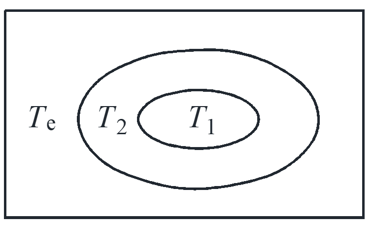
\[\left\{ \begin{array}{l}
\frac{{d{T_1}}}{{dt}} = a\left( {{T_2} – {T_1}} \right)\\
\frac{{d{T_2}}}{{dt}} = a\left( {{T_1} – {T_2}} \right) + b\left( {{T_e} – {T_2}} \right)
\end{array} \right.\]
\[\left\{ \begin{array}{l}
T_1^{\prime} = – a{T_1} + 2{T_2}\\
T_2^{\prime} = a{T_1} – \left( {a + b} \right){T_2} + b{T_e}
\end{array} \right.\]
\[a = 2,b = 3, T_e=0 \to \left\{ \begin{array}{l}
T_1^{\prime} = – 2{T_1} + 2{T_2}\\
T_2^{\prime} = 2{T_1} – 5{T_2}
\end{array} \right.,{T_1}\left( 0 \right) = 40,{T_2}\left( 0 \right) = 45\]
Eliminate variables
\[{T_2} = \frac{{T_1^{\prime} + 2{T_1}}}{2} \to {\left( {\frac{{T_1^{\prime} + 2{T_1}}}{2}} \right)^{\prime}} = 2{T_1} – 5\left( {\frac{{T_1^{\prime} + 2{T_1}}}{2}} \right)\]
\[T_1^{\prime\prime} + 7T_1^{\prime} + 6{T_1} = 0 \to {r^2} + 7r + 6 = 0\]
\[\left\{ \begin{array}{l}
{T_1} = {c_1}{e^{ – t}} + {c_2}{e^{ – 6t}}\\
{T_2} = \frac{1}{2}{c_1}{e^{ – t}} – 2{c_2}{e^{ – 6t}}
\end{array} \right. \to \left\{ \begin{array}{l}
{T_1} = 50{e^{ – t}} – 10{e^{ – 6t}}\\
{T_2} = 25{e^{ – t}} + 20{e^{ – 6t}}
\end{array} \right.\]
Autonomous system
\[\left\{ \begin{array}{l}
{x^{\prime}} = f\left( {x,y} \right)\\
{y^{\prime}} = g\left( {x,y} \right)
\end{array} \right. \to \left\{ \begin{array}{l}
x = x\left( t \right)\\
y = y\left( t \right)
\end{array} \right.\]
A system of the first-order autonomous ODE = velocity field.
Solution: parameterised curve with the right velocity everywhere.
Homogeneous ODE system
\[\left\{ \begin{array}{l}
{x^{\prime}} = – 2x + 2y\\
{y^{\prime}} = 2x – 5y
\end{array} \right. \to \left\{ \begin{array}{l}
x = {c_1}{e^{ – t}} + {c_2}{e^{ – 6t}}\\
y = \frac{1}{2}{c_1}{e^{ – t}} – 2{c_2}{e^{ – 6t}}
\end{array} \right.\]
Write the ODE system and the solution as follow
\[\left\{ \begin{array}{l}
{x^{\prime}}\\
{y^{\prime}}
\end{array} \right\} = \left[ {\begin{array}{*{20}{c}}
{ – 2}&2\\
2&{ – 5}
\end{array}} \right]\left\{ \begin{array}{l}
x\\
y
\end{array} \right\} \to \left\{ \begin{array}{l}
x\\
y
\end{array} \right\} = {c_1}\left\{ \begin{array}{l}
1\\
1/2
\end{array} \right\}{e^{ – t}} + {c_2}\left\{ \begin{array}{l}
1\\
– 2
\end{array} \right\}{e^{ – 6t}}\]
The trial solution is
\[\left\{ \begin{array}{l}
x\\
y
\end{array} \right\} = \left\{ \begin{array}{l}
{a_1}\\
{a_2}
\end{array} \right\}{e^{\lambda t}}\]
substitute the trial solution into the system
\[\lambda \left\{ \begin{array}{l}
{a_1}\\
{a_2}
\end{array} \right\}{e^{\lambda t}} = \left[ {\begin{array}{*{20}{c}}
{ – 2}&2\\
2&{ – 5}
\end{array}} \right]\left\{ \begin{array}{l}
{a_1}\\
{a_2}
\end{array} \right\}{e^{\lambda t}}\]
\[\left\{ \begin{array}{l}
\lambda {a_1} = – 2{a_1} + 2{a_2}\\
\lambda {a_2} = 2{a_1} – 5{a_2}
\end{array} \right. \to \left\{ \begin{array}{l}
\left( { – 2 – \lambda } \right){a_1} + 2{a_2} = 0\\
2{a_1} + \left( { – 5 – \lambda } \right){a_2} = 0
\end{array} \right.\]
\[\rm{nontrivail = nonzero \ solution} \Leftrightarrow \left| {\begin{array}{*{20}{c}}
{ – 2 – \lambda }&2\\
2&{ – 5 – \lambda }
\end{array}} \right| = 0\]
\[\left( {\lambda + 2} \right)\left( {\lambda + 5} \right) – 4 = 0 \to {\lambda ^2} + 7\lambda + 6 = 0\]
This equation about \(\lambda\) is the same as we derived by eliminating variables, this equation is called characteristic equation.
\[\lambda = 1 \to \left\{ \begin{array}{l}
– {a_1} + 2{a_2} = 0\\
2{a_1} – 4{a_2} = 0
\end{array} \right. \to \left\{ \begin{array}{l}
{a_1} = 2\\
{a_2} = 1
\end{array} \right. \to \left\{ \begin{array}{l}
2\\
1
\end{array} \right\}{e^{ – t}}\]
\[\lambda = – 6 \to \left\{ \begin{array}{l}
4{a_1} + 2{a_2} = 0\\
2{a_1} + 1{a_2} = 0
\end{array} \right. \to \left\{ \begin{array}{l}
{a_1} = 1\\
{a_2} = – 2
\end{array} \right. \to \left\{ \begin{array}{l}
1\\
– 2
\end{array} \right\}{e^{ – 6t}}\]
superposition
\[{{\tilde c}_1}\left\{ \begin{array}{l}
2\\
1
\end{array} \right\}{e^{ – t}} + {{\tilde c}_2}\left\{ \begin{array}{l}
1\\
– 2
\end{array} \right\}{e^{ – 6t}} \to {{\tilde c}_1} = {c_1}/2,{{\tilde c}_2} = {c_2}\]
Solution method in general:
\[{\left\{ \begin{array}{l}
x\\
y
\end{array} \right\}^{\prime}} = \left[ {\begin{array}{*{20}{c}}
a&b\\
c&d
\end{array}} \right]\left\{ \begin{array}{l}
x\\
y
\end{array} \right\}\]
\[A = \left[ {\begin{array}{*{20}{c}}
a&b\\
c&d
\end{array}} \right],\left| {A – \lambda I} \right| = \left| {\begin{array}{*{20}{c}}
{a – \lambda }&b\\
c&{d – \lambda }
\end{array}} \right| = 0\]
Characteristic equation of matrix \(A\)
\[{\lambda ^2} – \left( {a + d} \right)\lambda + \left( {ad + bc} \right) = 0\]
\[tr\left( A \right) = a + d,\det \left( A \right) = ad + bc\]
Eigenvalues: the real and distinct roots \({\lambda _1},{\lambda _2}\), sometimes also called characteristic values or proper values.
the general solution is then
\[\left\{ \begin{array}{l}
x\\
y
\end{array} \right\} = {c_1}\left\{ \begin{array}{l}
{a_{11}}\\
{a_{21}}
\end{array} \right\}{e^{{\lambda _1}t}} + {c_2}\left\{ \begin{array}{l}
{a_{12}}\\
{a_{22}}
\end{array} \right\}{e^{{\lambda _2}t}}\]
Summary for the procedure of solving ODE system
\[{\overrightarrow X ^{\prime}} = A\overrightarrow X \]
- \(\left| {A – \lambda I} \right| = 0\), roots \({\lambda _1},{\lambda _2}, \cdot \cdot \cdot \) eigenvalue
- \(\left( {A – \lambda I} \right)\overrightarrow \alpha = \overrightarrow 0 \), find \({\overrightarrow \alpha _1},{\overrightarrow \alpha _1}, \cdot \cdot \cdot \) eigenvector
- \(\overrightarrow X = \sum {{c_i}} {\overrightarrow \alpha _i}{e^{{\lambda _i}t}}\)
Example:
\(X_i\) = temperature in tank \(i\), find the functions of \({X_i}\left( t \right)\)
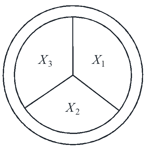
\[\left\{ \begin{array}{l}
X_1^{\prime} = – 2{X_1} + {X_2} + {X_3}\\
X_2^{\prime} = {X_1} – 2{X_2} + {X_3}\\
X_3^{\prime} = {X_1} + {X_2} – 2{X_3}
\end{array} \right.\]
\[\left| {A – \lambda I} \right| = \left| {\begin{array}{*{20}{c}}
{ – 2 – \lambda }&1&1\\
1&{ – 2 – \lambda }&1\\
1&1&{ – 2 – \lambda }
\end{array}} \right| = \lambda {\left( {\lambda + 3} \right)^2} = 0\]
\[\lambda = 0 \to \left\{ \begin{array}{l}
– 2{a_1} + {a_2} + {a_3} = 0\\
{a_1} – 2{a_2} + {a_3} = 0\\
{a_1} + {a_2} – 2{a_3} = 0
\end{array} \right. \to \left( \begin{array}{l}
1\\
1\\
1
\end{array} \right){e^{0t}}\]
\[\lambda = – 3 \to \left\{ \begin{array}{l}
{a_1} + {a_2} + {a_3} = 0\\
{a_1} + {a_2} + {a_3} = 0\\
{a_1} + {a_2} + {a_3} = 0
\end{array} \right. \to \left( {\begin{array}{*{20}{c}}
0\\
0\\
{ – 1}
\end{array}} \right){e^{ – 3t}},\left( {\begin{array}{*{20}{c}}
0\\
{ – 1}\\
0
\end{array}} \right){e^{ – 3t}}\]
\[\left( \begin{array}{l}
{X_1}\\
{X_2}\\
{X_3}
\end{array} \right) = {c_1}\left( {\begin{array}{*{20}{c}}
0\\
0\\
{ – 1}
\end{array}} \right){e^{ – 3t}} + {c_2}\left( {\begin{array}{*{20}{c}}
0\\
{ – 1}\\
0
\end{array}} \right){e^{ – 3t}} + {c_3}\left( \begin{array}{l}
1\\
1\\
1
\end{array} \right)\]
complete eigenvalue: \(\lambda \) is repeated eigenvalue, but you can find enough independent eigenvectors to make up needed number of independent solutions
defective eigenvalue: single root
\(A\) is real \(n \times n\) matrix which is symmetric, \({A^T} = A\) \( \Rightarrow \) all its eigenvalue are complete.
Complex eigenvalues
calculate the complex eigenvectors and take the real part
Example:
\[\left\{ \begin{array}{l}
{x^{\prime}} = x + 2y\\
{y^{\prime}} = – x – y
\end{array} \right. \to \lambda = \pm i\]
\[\lambda = i \to \left\{ \begin{array}{l}
\left( {1 – i} \right){a_1} + 2{a_2} = 0\\
– {a_1} + \left( { – 1 – i} \right){a_2} = 0
\end{array} \right. \to \left( \begin{array}{l}
{a_1}\\
{a_2}
\end{array} \right) = \left( {\begin{array}{*{20}{c}}
1\\
{ – \frac{{1 – i}}{2}}
\end{array}} \right)\]
\[\left( {\begin{array}{*{20}{c}}
1\\
{ – \frac{{1 – i}}{2}}
\end{array}} \right){e^{it}} = \left[ {\left( {\begin{array}{*{20}{c}}
1\\
{ – \frac{1}{2}}
\end{array}} \right) + \left( {\begin{array}{*{20}{c}}
0\\
{\frac{i}{2}}
\end{array}} \right)} \right]\left( {\cos t + i\sin t} \right) \to \left( \begin{array}{l}
x\\
y
\end{array} \right) = \left( {\begin{array}{*{20}{c}}
{\cos t}\\
{ – \frac{1}{2}\left( {\cos t + \sin t} \right)}
\end{array}} \right)\]
Sketch solutions of ODE system
\[{\left\{ \begin{array}{l}
x\\
y
\end{array} \right\}^{\prime}} = \left[ {\begin{array}{*{20}{c}}
a&b\\
c&d
\end{array}} \right]\left\{ \begin{array}{l}
x\\
y
\end{array} \right\}\]
- four easy solutions \({c_1} = \pm 1,{c_2} = 0;{c_1} = 0,{c_2} = \pm 1\)
- fill in the rest
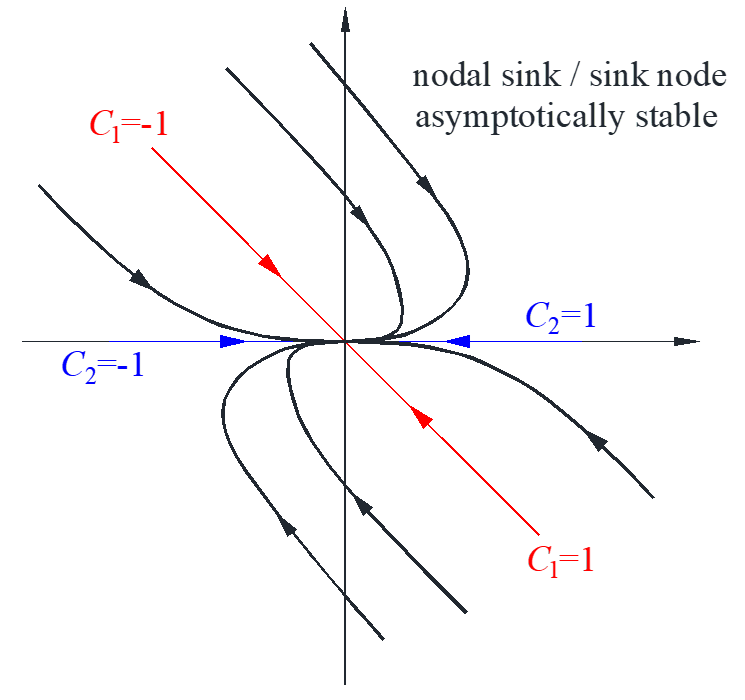
Situation #1
\[\left\{ \begin{array}{l}
{x^{\prime}} = – x + 2y\\
{y^{\prime}} = – 3y
\end{array} \right. \to \left\{ \begin{array}{l}
x = {c_1}{e^{ – 3t}} + {c_2}{e^{ – t}}\\
y = – {c_1}{e^{ – 3t}}
\end{array} \right.\]
\[\left\{ \begin{array}{l}
x\\
y
\end{array} \right\} = \underbrace {{c_1}\left( {\begin{array}{*{20}{c}}
1\\
{ – 1}
\end{array}} \right){e^{ – 3t}}}_{{\rm{dominantas}}t \to – \infty } + \underbrace {{c_2}\left( {\begin{array}{*{20}{c}}
1\\
0
\end{array}} \right){e^{ – t}}}_{{\rm{dominantas}}t \to \infty }\]
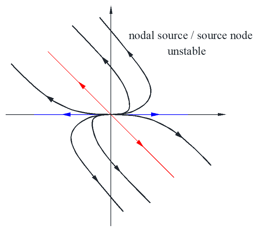
Situation #2
\[\left\{ \begin{array}{l}
x\\
y
\end{array} \right\} = {c_1}\left( {\begin{array}{*{20}{c}}
1\\
{ – 1}
\end{array}} \right){e^{3t}} + {c_2}\left( {\begin{array}{*{20}{c}}
1\\
0
\end{array}} \right){e^t}\]
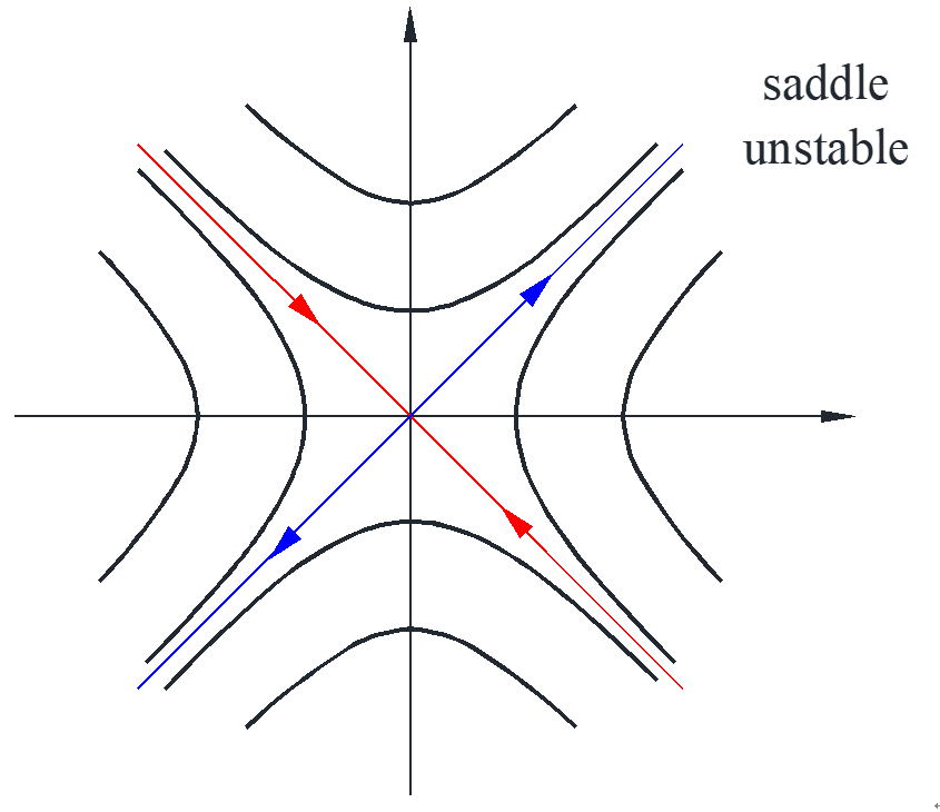
Situation #3
\[\left\{ \begin{array}{l}
{x^{\prime}} = – x + 3y\\
{y^{\prime}} = 5x – 3y
\end{array} \right. \to \left\{ \begin{array}{l}
x\\
y
\end{array} \right\} = {c_1}\left( {\begin{array}{*{20}{c}}
3\\
{ – 5}
\end{array}} \right){e^{ – 6t}} + {c_2}\left( {\begin{array}{*{20}{c}}
1\\
1
\end{array}} \right){e^{2t}}\]
Situation #4
\[\left\{ \begin{array}{l}
{x^{\prime}} = – x – y\\
{y^{\prime}} = 2x – 3y
\end{array} \right. \to \left\{ \begin{array}{l}
x\\
y
\end{array} \right\} = \underbrace {\left[ {{c_1}\left( {\begin{array}{*{20}{c}}
{{a_1}}\\
{{a_2}}
\end{array}} \right)\cos t + {c_2}\left( {\begin{array}{*{20}{c}}
{{b_1}}\\
{{b_2}}
\end{array}} \right)\sin t} \right]}_{{\rm{bounded,period}} = 2\pi }{e^{ – 2t}}\]
the bounded part must satisfies \(A{x^2} + B{y^2} + Cxy = D\), which is an ellipse
How to determine whether the line is clockwise or counterclockwise? Choose one point and calculate the vector, for example at point \(\left( {1,0} \right)\), \({x^{\prime}} = – 1,{y^{\prime}} = 2\), the vector at this point is shown as the red line.
Inhomogeneous ODE system
\[{\overrightarrow X ^{\prime}} = A\overrightarrow X \]
Theorem #1: the general solution to \({\overrightarrow X ^{\prime}} = A\overrightarrow X \) is \(\overrightarrow X = {c_1}{\overrightarrow X _1} + {c_2}{\overrightarrow X _2}\), where \({\overrightarrow X _1}\) and \({\overrightarrow X _2}\) are two linearly independent solutions.
Theorem #2: Wronskian of two solutions
\[W\left( {{{\overrightarrow X }_1},{{\overrightarrow X }_2}} \right) = \left| {{{\overrightarrow X }_1},{{\overrightarrow X }_2}} \right| = \left\{ \begin{array}{l}
0 \qquad \qquad \qquad \qquad {\overrightarrow X _1},{\overrightarrow X _2} \ {\rm{are \ dependent}}\\
{\rm{never}}\ 0\ {\rm{for \ any}}\ t \quad \ \ \ \ \ {\overrightarrow X _1},{\overrightarrow X _2} \ {\rm{are \ independent}}
\end{array} \right.\]
Fundamental matrix for \({\overrightarrow X ^{\prime}} = A\overrightarrow X \)
\[\overline {\underline X } = \left[ {{{\overrightarrow X }_1},{{\overrightarrow X }_2}} \right] \qquad {\overrightarrow X _1},{\overrightarrow X _2}\ {\rm{are\ independent \ solution}}\]
properties:
#1 \(\left| {\overline {\underline X } } \right| \ne 0\) for any \(t\)
#2 \({\overline {\underline X } ^{\prime}} = A\overline {\underline X } \Leftrightarrow \left[ {\overrightarrow X _1^{\prime},\overrightarrow X _2^{\prime}} \right] = A\left[ {{{\overrightarrow X }_1},{{\overrightarrow X }_2}} \right] \Leftrightarrow \overrightarrow X _1^{\prime} = A{\overrightarrow X _1},\overrightarrow X _2^{\prime} = A{\overrightarrow X _2}\)
Theorem #3: for inhomogeneous system \({\overrightarrow X ^{\prime}} = A\overrightarrow X + \overrightarrow r \left( t \right)\), the solution is \(\overrightarrow X = {\overrightarrow X _c} + {\overrightarrow X _p}\)
method for particular solution: variation of parameters
\[{\overrightarrow X _p} = {v_1}\left( t \right){\overrightarrow X _1} + {v_2}\left( t \right){\overrightarrow X _2} = \overline {\underline X } \overrightarrow v \]
substitute into the system to get the \(\overrightarrow v \)
\[{\overrightarrow X ^{\prime}} = A\overrightarrow X + \overrightarrow r \to {\overline {\underline X } ^{\prime}}\overrightarrow v + \overline {\underline X } {\overrightarrow v ^{\prime}} = A\overline {\underline X } \overrightarrow v + \overrightarrow r \]
\[{\overline {\underline X } ^{\prime}} = A\overline {\underline X } \to \overline {\underline X } {\overrightarrow v ^{\prime}} = \overrightarrow r \to {\overrightarrow v ^{\prime}} = {\overline {\underline X } ^{ – 1}}\overrightarrow r \]
\[\overrightarrow v = \int {{{\overline {\underline X } }^{ – 1}}\overrightarrow r dt} \to {\overrightarrow X _p} = \overline {\underline X } \int {{{\overline {\underline X } }^{ – 1}}\overrightarrow r dt} \]
Example: mixing problem
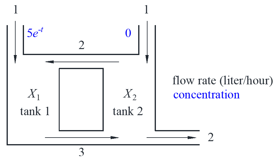
\[\left\{ \begin{array}{l}
x_1^{\prime} = – 3{x_1} + 2{x_2} + 5{e^{ – t}}\\
x_2^{\prime} = 3{x_1} – 4{x_2} + 0
\end{array} \right.\]
\[{\overrightarrow X _c} = {c_1}\left( {\begin{array}{*{20}{c}}
1\\
1
\end{array}} \right){e^{ – t}} + {c_2}\left( {\begin{array}{*{20}{c}}
2\\
{ – 3}
\end{array}} \right){e^{ – 6t}}\]
\[\overline {\underline X } = \left[ {\begin{array}{*{20}{c}}
{{e^{ – t}}}&{2{e^{ – 6t}}}\\
{{e^{ – t}}}&{ – 3{e^{ – 6t}}}
\end{array}} \right],{\overline {\underline X } ^{ – 1}}\overrightarrow r = \left[ {\begin{array}{*{20}{c}}
{\frac{3}{5}{e^t}}&{\frac{2}{5}{e^t}}\\
{\frac{1}{5}{e^{6t}}}&{ – \frac{1}{5}{e^{6t}}}
\end{array}} \right]\left( {\begin{array}{*{20}{c}}
{5{e^{ – t}}}\\
0
\end{array}} \right) = \left( {\begin{array}{*{20}{c}}
3\\
{{e^{5t}}}
\end{array}} \right)\]
\[{\overrightarrow X _p} = \overline {\underline X } \int {{{\overline {\underline X } }^{ – 1}}\overrightarrow r dt} = \overline {\underline X } \int {\left( {\begin{array}{*{20}{c}}
3\\
{{e^{5t}}}
\end{array}} \right)dt} = \left[ {\begin{array}{*{20}{c}}
{{e^{ – t}}}&{2{e^{ – 6t}}}\\
{{e^{ – t}}}&{ – 3{e^{ – 6t}}}
\end{array}} \right]\left( {\begin{array}{*{20}{c}}
{3t}\\
{\frac{1}{5}{e^{5t}}}
\end{array}} \right) = \left( {\begin{array}{*{20}{c}}
{3t{e^{ – t}} + \frac{2}{5}{e^{ – t}}}\\
{3t{e^{ – t}} – \frac{3}{5}{e^{ – t}}}
\end{array}} \right)\]
\[\overrightarrow X = {c_1}\left( {\begin{array}{*{20}{c}}
1\\
1
\end{array}} \right){e^{ – t}} + {c_2}\left( {\begin{array}{*{20}{c}}
2\\
{ – 3}
\end{array}} \right){e^{ – 6t}} + \left( {\begin{array}{*{20}{c}}
{3t{e^{ – t}} + \frac{2}{5}{e^{ – t}}}\\
{3t{e^{ – t}} – \frac{3}{5}{e^{ – t}}}
\end{array}} \right)\]
Matrix exponential
\[{\overrightarrow X ^{\prime}} = A\overrightarrow X \]
1*1 case: \({x^{\prime}} = ax \to x = c{e^{at}}\)
\[{e^{at}} = 1 + at + \frac{{{a^2}{t^2}}}{{2!}} + \frac{{{a^3}{t^3}}}{{3!}} + \cdot \cdot \cdot \]
\[\frac{{d{e^{at}}}}{{dt}} = a + {a^2}t + \frac{{{a^3}{t^2}}}{{2!}} + \cdot \cdot \cdot = a{e^{at}}\]
So, a fundamental matrix for \({\overrightarrow X ^{\prime}} = A\overrightarrow X \) is \({e^{At}}\), satisfying \({\overline {\underline X } ^{\prime}} = A\overline {\underline X } \) and \(\left| {\overline {\underline X } \left( 0 \right)} \right| = \left| I \right| = 1 \ne 0\).
Example:
\[\left\{ \begin{array}{l}
{x^{\prime}} = y\\
{y^{\prime}} = x
\end{array} \right. \to {\overrightarrow X ^{\prime}} = A\overrightarrow X ,A = \left[ {\begin{array}{*{20}{c}}
0&1\\
1&0
\end{array}} \right]\]
\[{A^2} = \left[ {\begin{array}{*{20}{c}}
0&1\\
1&0
\end{array}} \right]\left[ {\begin{array}{*{20}{c}}
0&1\\
1&0
\end{array}} \right] = \left[ {\begin{array}{*{20}{c}}
1&0\\
0&1
\end{array}} \right] = I,{A^3} = A,{A^4} = I, \cdot \cdot \cdot \]
\begin{align*}
{e^{At}} &= I + At + \frac{{{A^2}{t^2}}}{{2!}} + \frac{{{A^3}{t^3}}}{{3!}} + \cdot \cdot \cdot = \left[ {\begin{array}{*{20}{c}}
{1 + \frac{{{t^2}}}{2} + \frac{{{t^4}}}{{4!}} + \cdot \cdot \cdot }&{t + \frac{{{t^3}}}{{3!}} + \frac{{{t^5}}}{{5!}} + \cdot \cdot \cdot }\\
{t + \frac{{{t^3}}}{{3!}} + \frac{{{t^5}}}{{5!}} + \cdot \cdot \cdot }&{1 + \frac{{{t^2}}}{2} + \frac{{{t^4}}}{{4!}} + \cdot \cdot \cdot }
\end{array}} \right]\\
&= \left[ {\begin{array}{*{20}{c}}
{\cosh t}&{\sinh t}\\
{\sinh t}&{\cosh t}
\end{array}} \right] = \frac{1}{2}\left[ {\begin{array}{*{20}{c}}
{{e^t} + {e^{ – t}}}&{{e^t} – {e^{ – t}}}\\
{{e^t} – {e^{ – t}}}&{{e^t} + {e^{ – t}}}
\end{array}} \right]
\end{align*}
IVP (initial value problem)
\[{\overrightarrow X ^{\prime}} = A\overrightarrow X ,\overrightarrow X \left( 0 \right) = {\overrightarrow X _0}\]
\[\overrightarrow X = {e^{At}}\overrightarrow C ,\overrightarrow X \left( 0 \right) = {e^{A0}}\overrightarrow C = \overrightarrow C \to \overrightarrow X = {e^{At}}\overrightarrow C {\overrightarrow X _0}\]
In general, \({e^{A + B}} \ne {e^A}{e^B}\), only true in special case \(AB = BA\)
- \(A = cI\)
- \(B = – A \to {e^{A\left( { – A} \right)}} = {e^A}{e^{ – A}} = I \Leftrightarrow {\left( {{e^A}} \right)^{ – 1}} = {e^{ – A}}\)
- \(B = {A^{ – 1}}\)
Methods to calculate \({e^{At}}\)
#1 series: too hard
\[{e^{At}} = I + At + \frac{{{A^2}{t^2}}}{{2!}} + \frac{{{A^3}{t^3}}}{{3!}} + \cdot \cdot \cdot \]
# 2 exponential law: only useful for symmetric matrix
\[\left[ {\begin{array}{*{20}{c}}
a&b\\
b&c
\end{array}} \right] = \left[ {\begin{array}{*{20}{c}}
a&0\\
0&c
\end{array}} \right] + \left[ {\begin{array}{*{20}{c}}
0&b\\
b&0
\end{array}} \right]\]
#3 all other cases: \({e^{At}} = \overline {\underline X } \cdot {\overline {\underline X } ^{ – 1}}\left( 0 \right)\)
\(\overline {\underline X } \cdot {\overline {\underline X } ^{ – 1}}\left( 0 \right)\) is still a fundamental matrix, and \(\overline {\underline X } \left( 0 \right) \cdot {\overline {\underline X } ^{ – 1}}\left( 0 \right) = I = {e^{At}}\left( 0 \right)\). \({e^{At}}\) has the same two properties.
For example above
\[\left\{ \begin{array}{l}
{x^{\prime}} = y\\
{y^{\prime}} = x
\end{array} \right. \to \overrightarrow X = {c_1}\left( {\begin{array}{*{20}{c}}
1\\
1
\end{array}} \right){e^t} + {c_2}\left( {\begin{array}{*{20}{c}}
1\\
{ – 1}
\end{array}} \right){e^{ – t}}\]
\[\overline {\underline X } = \left[ {\begin{array}{*{20}{c}}
{{e^t}}&{{e^{ – t}}}\\
{{e^t}}&{ – {e^{ – t}}}
\end{array}} \right],\overline {\underline X } \left( 0 \right) = \left[ {\begin{array}{*{20}{c}}
1&1\\
1&{ – 1}
\end{array}} \right],{\overline {\underline X } ^{ – 1}}\left( 0 \right) = \frac{1}{2}\left[ {\begin{array}{*{20}{c}}
1&1\\
1&{ – 1}
\end{array}} \right]\]
\[{e^{At}} = \overline {\underline X } \cdot {\overline {\underline X } ^{ – 1}}\left( 0 \right) = \left[ {\begin{array}{*{20}{c}}
{{e^t}}&{{e^{ – t}}}\\
{{e^t}}&{ – {e^{ – t}}}
\end{array}} \right] \cdot \frac{1}{2}\left[ {\begin{array}{*{20}{c}}
1&1\\
1&{ – 1}
\end{array}} \right] = \frac{1}{2}\left[ {\begin{array}{*{20}{c}}
{{e^t} + {e^{ – t}}}&{{e^t} – {e^{ – t}}}\\
{{e^t} – {e^{ – t}}}&{{e^t} + {e^{ – t}}}
\end{array}} \right]\]
Decoupling
\[\left\{ \begin{array}{l}
u = ax + by\\
v = cx + dy
\end{array} \right. \to \left\{ \begin{array}{l}
{u^{\prime}} = {k_1}u\\
{v^{\prime}} = {k_2}v
\end{array} \right.\]
Decouple: only when eigenvalues are real and complete
\(A\) is symmetric \( \to \) eigenvalues are always real and complete \( \to \) can always decouple
\[\left( {\begin{array}{*{20}{c}}
u\\
v
\end{array}} \right) = \left[ {\begin{array}{*{20}{c}}
{a_1^{\prime}}&{a_2^{\prime}}\\
{b_1^{\prime}}&{b_2^{\prime}}
\end{array}} \right]\left( {\begin{array}{*{20}{c}}
x\\
y
\end{array}} \right) \to D = \left[ {\begin{array}{*{20}{c}}
{a_1^{\prime}}&{a_2^{\prime}}\\
{b_1^{\prime}}&{b_2^{\prime}}
\end{array}} \right]{\rm{decouple \ matrix}}\]
\[\left( {\begin{array}{*{20}{c}}
x\\
y
\end{array}} \right) = \left[ {\begin{array}{*{20}{c}}
{{a_1}}&{{a_2}}\\
{{b_1}}&{{b_2}}
\end{array}} \right]\left( {\begin{array}{*{20}{c}}
u\\
v
\end{array}} \right) \to E = {D^{ – 1}} = \left[ {\begin{array}{*{20}{c}}
{{a_1}}&{{a_2}}\\
{{b_1}}&{{b_2}}
\end{array}} \right] = \left[ {\begin{array}{*{20}{c}}
{{{\overrightarrow \alpha }_1}}&{{{\overrightarrow \alpha }_2}}
\end{array}} \right]\]
The columns of \(E\) are the two eigenvectors. Substitute into \({\overrightarrow X ^{\prime}} = A\overrightarrow X \) to see if decoupled in \(uv\) system:
\[\left( {A – {\lambda _i}I} \right){\overrightarrow \alpha _i} = \overrightarrow 0 \to A{\overrightarrow \alpha _i} = {\lambda _i}\overrightarrow \alpha _i \]
The left side of the equation \(A{\overrightarrow \alpha _i}\) can be seen as a linear transformation to a plane so that every vector in this plane goes to a different direction with different value. The right side \({\lambda _i}{\overrightarrow \alpha _i}\) can be seen as a vector \({\overrightarrow \alpha _i}\) is just shrunk or stretched with a factor \({\lambda _i}\).
\begin{align*}
AE &= A\left[ {\begin{array}{*{20}{c}}
{{{\overrightarrow \alpha }_1}}&{{{\overrightarrow \alpha }_2}}
\end{array}} \right] = \left[ {\begin{array}{*{20}{c}}
{A{{\overrightarrow \alpha }_1}}&{A{{\overrightarrow \alpha }_2}}
\end{array}} \right] = \left[ {\begin{array}{*{20}{c}}
{{\lambda _1}{{\overrightarrow \alpha }_1}}&{{\lambda _2}{{\overrightarrow \alpha }_2}}
\end{array}} \right]\\
&= \left[ {\begin{array}{*{20}{c}}
{{{\overrightarrow \alpha }_1}}&{{{\overrightarrow \alpha }_2}}
\end{array}} \right]\left[ {\begin{array}{*{20}{c}}
{{\lambda _1}}&0\\
0&{{\lambda _2}}
\end{array}} \right] = E\left[ {\begin{array}{*{20}{c}}
{{\lambda _1}}&0\\
0&{{\lambda _2}}
\end{array}} \right]
\end{align*}
\[\overrightarrow X = E\overrightarrow u \to {\overrightarrow X ^{\prime}} = E{\overrightarrow u ^{\prime}},A\overrightarrow X = AE\overrightarrow u \]
\[E{\overrightarrow u ^{\prime}} = AE\overrightarrow u = E\left[ {\begin{array}{*{20}{c}}
{{\lambda _1}}&0\\
0&{{\lambda _2}}
\end{array}} \right]\overrightarrow u \to {\overrightarrow u ^{\prime}} = \left[ {\begin{array}{*{20}{c}}
{{\lambda _1}}&0\\
0&{{\lambda _2}}
\end{array}} \right]\overrightarrow u \]
\[\left\{ \begin{array}{l}
{u^{\prime}} = {\lambda _1}u\\
{v^{\prime}} = {\lambda _2}v
\end{array} \right. \to \left\{ \begin{array}{l}
u = {c_1}{e^{{\lambda _1}t}}\\
v = {c_2}{e^{{\lambda _2}t}}
\end{array} \right.\]
Example:
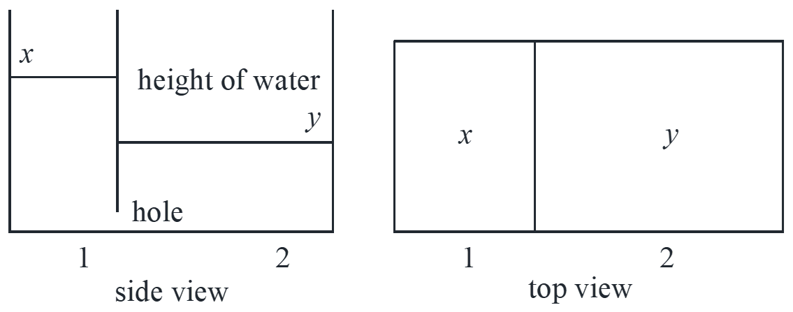
flow rate through the hole (mL/s) \( \propto \) area of hole \( \cdot \) height difference
height difference \( \propto \) pressure at hole
\[\left\{ \begin{array}{l}
{x^{\prime}} = c\left( {y – x} \right)\\
2{y^{\prime}} = c\left( {x – y} \right)
\end{array} \right.\mathop \to \limits_{c = 2} \left\{ \begin{array}{l}
{x^{\prime}} = – 2x + 2y\\
{y^{\prime}} = x – y
\end{array} \right.\]
Decouple with physical meaning
We need to find more natural variables: #1: difference of height proportional to water pressure \(x – y\) ; #2: constant variable in the system, the total water \(x + 2y\).
\[\left\{ \begin{array}{l}
u = x + 2y\\
v = x – y
\end{array} \right. \to \left\{ \begin{array}{l}
{u^{\prime}} = {x^{\prime}} + 2{y^{\prime}} = 0\\
{v^{\prime}} = {x^{\prime}} – {y^{\prime}} = – 3x + 3y = – 3v
\end{array} \right. \to \left\{ \begin{array}{l}
u = {c_1}\\
v = {c_2}{e^{ – 3t}}
\end{array} \right.\]
\[\left\{ \begin{array}{l}
u = x + 2y\\
v = x – y
\end{array} \right. \to \left\{ \begin{array}{l}
x = \frac{1}{3}\left( {u + 2v} \right) = \frac{1}{3}\left( {{c_1} + 2{c_2}{e^{ – 3t}}} \right)\\
y = \frac{1}{3}\left( {u – v} \right) = \frac{1}{3}\left( {{c_1} – {c_2}{e^{ – 3t}}} \right)
\end{array} \right.\]
\[\overrightarrow X = \frac{1}{3}{c_1}\left( {\begin{array}{*{20}{c}}
1\\
1
\end{array}} \right) + \frac{1}{3}{c_2}\left( {\begin{array}{*{20}{c}}
2\\
{ – 1}
\end{array}} \right){e^{ – 3t}}\]
decouple with systematical method
\[\left\{ \begin{array}{l}
{x^{\prime}} = – 2x + 2y\\
{y^{\prime}} = x – y
\end{array} \right. \to \overrightarrow X = {c_1}\left( {\begin{array}{*{20}{c}}
1\\
1
\end{array}} \right) + {c_2}\left( {\begin{array}{*{20}{c}}
{ – 2}\\
1
\end{array}} \right){e^{ – 3t}}\]
\[E = \left[ {\begin{array}{*{20}{c}}
1&{ – 2}\\
1&1
\end{array}} \right],D = {E^{ – 1}} = \frac{1}{3}\left[ {\begin{array}{*{20}{c}}
1&2\\
{ – 1}&1
\end{array}} \right]\]
\[\left\{ \begin{array}{l}
u = \frac{1}{3}x + \frac{2}{3}y\\
v = – \frac{1}{3}x + \frac{1}{3}y
\end{array} \right. \to \left\{ \begin{array}{l}
{u^{\prime}} = \frac{1}{3}{x^{\prime}} + \frac{2}{3}{y^{\prime}} = 0\\
{v^{\prime}} = – \frac{1}{3}{x^{\prime}} + \frac{1}{3}{y^{\prime}} = x – y = – v
\end{array} \right.\]
The only difference between the \(u,v\) chosen by physical meaning is the coefficient, actually they are the same.
Sketch trajectory
\[{\rm{autonomous \ nonlinear}}\left\{ \begin{array}{l}
{x^{\prime}} = f\left( {x,y} \right)\\
{y^{\prime}} = g\left( {x,y} \right)
\end{array} \right.\]
Example: nonlinear pendulum with light damp
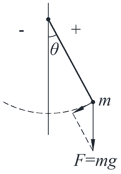
\[m\overrightarrow a = \overrightarrow F \to ml{\theta ^{\prime\prime}} = – mg\sin \theta – {c_1}l{\theta ^{\prime}}\]
\[{\theta ^{\prime\prime}} + \frac{{{c_1}}}{m}{\theta ^{\prime}} + \frac{l}{g}\sin \theta = 0 \to {\theta ^{\prime\prime}} + c{\theta ^{\prime}} + k\sin \theta = 0\]
Assume \({c = 1,k = 2}\) and introduce \(\omega \):
\[{\theta ^{\prime\prime}} + {\theta ^{\prime}} + 2\sin \theta = 0 \to \left\{ \begin{array}{l}
{\theta ^{\prime}}=\omega\\
{\omega ^{\prime}} = – 2\sin \theta – \omega
\end{array} \right.\]
#1: Look for critical points of the system, which means the velocity vector is zero.
\[\left\{ \begin{array}{l}
\omega = 0\\
– 2\sin \theta – \omega = 0
\end{array} \right. \to \left\{ \begin{array}{l}
\omega = 0\\
\theta = 0, \pm \pi , \pm 2\pi , \cdots
\end{array} \right.\]
Physically speaking, there are only two critical points \(\left( {0,0} \right)\) and \(\left( {0,\pi } \right)\), and the point \(\left( {0,0} \right)\) is stable, point \(\left( {0,\pi } \right)\) is unstable.
#2: Linearize the system near each critical point and plot the trajectories of this linearized system near this critical point.
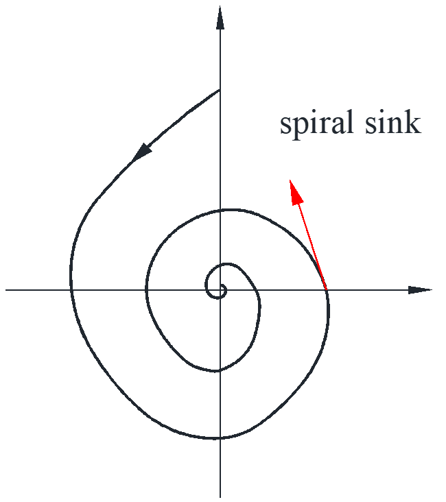
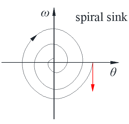
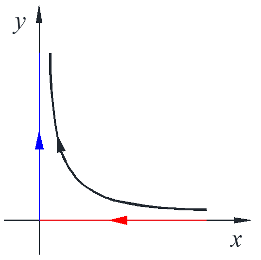
Linearize at \(\left( {0,0} \right)\)
\[\left\{ \begin{array}{l}
{\theta ^{\prime}} = \omega \\
{\omega ^{\prime}} = – 2\sin \theta – \omega \approx – 2\theta – \omega
\end{array} \right. \to \lambda = \frac{{ – 1 \pm \sqrt { – 7} }}{2}\]
With complex roots, the curve is a spiral because of the \(sin\) and \(cos\). Here the curve is spiral sink since \(\lambda = – \frac{1}{2} \pm bi\). At point \(\left( {1,0} \right)\), the velocity vector is \(\left( {0,-2} \right)\), the curve is clockwise as shown below.
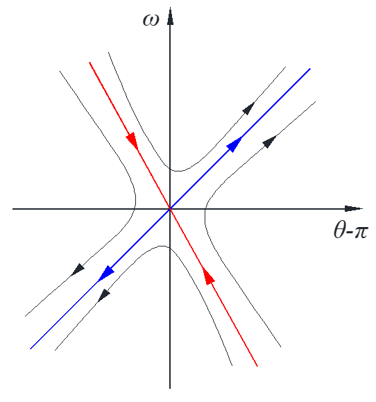
Linearize at \(\left( {\pi,0} \right)\)
calculate the Jacobian matrix at point \(\left( {\pi,0} \right)\)
\[J = \left[ {\begin{array}{*{20}{c}}
{{f_x}}&{{f_y}}\\
{{g_x}}&{{g_y}}
\end{array}} \right] = \left[ {\begin{array}{*{20}{c}}
{\frac{{\partial f}}{{\partial x}}}&{\frac{{\partial f}}{{\partial y}}}\\
{\frac{{\partial g}}{{\partial x}}}&{\frac{{\partial g}}{{\partial y}}}
\end{array}} \right] = \left[ {\begin{array}{*{20}{c}}
0&1\\
{ – 2\cos \theta }&{ – 1}
\end{array}} \right]\]
\[{\rm{at}}\ \left( {0,0} \right),J = \left[ {\begin{array}{*{20}{c}}
0&1\\
{ – 2}&{ – 1}
\end{array}} \right] \quad {\rm{same}}\]
\[{\rm{at}} \ \left( {0,\pi } \right),J = \left[ {\begin{array}{*{20}{c}}
0&1\\
2&{ – 1}
\end{array}} \right] \to \lambda = 1, – 2\]
\[\overrightarrow X = {c_1}\left( {\begin{array}{*{20}{c}}
1\\
1
\end{array}} \right){e^t} + {c_2}\left( {\begin{array}{*{20}{c}}
1\\
{ – 2}
\end{array}} \right){e^{ – 2t}}\]
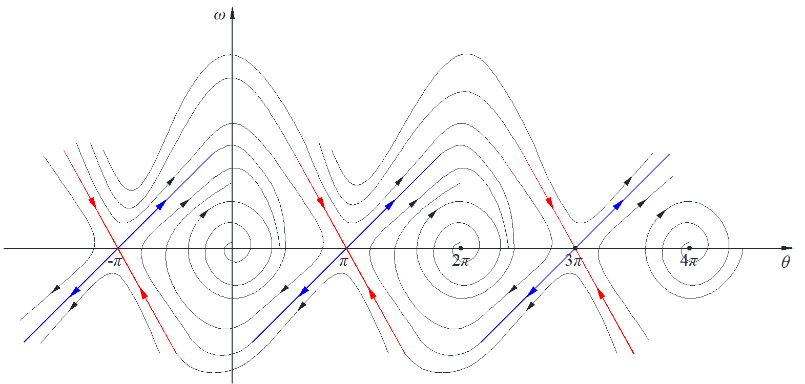
#3: big picture, plot trajectories around each critical point then add some
note: the trajectories cannot intersect with each other, so one curve cannot come across another.
Limit cycle and closed trajectory
Limit cycle: closed trajectory, isolated (no others nearby), stable
Existence problem
In general, not much is known and most are done by computer search. There is a Poincare-Bendixson theorem.
Non-existence Bendixson’s criteria:
\(D\) is the region of plane, \({f_x},{g_y}\) are continuous, if the divergence \(div\overrightarrow F = {f_x} + {g_y} \ne 0\) in \(D\), then there is no closed trajectory in \(D\).
Example:
\[\left\{ \begin{array}{l}
{x^{\prime}} = {x^3} + {y^3}\\
{y^{\prime}} = 3x + {y^3} + 2y
\end{array} \right. \to \overrightarrow F = {f_x} + {g_y} = 3{x^2} + 3{y^2} + 2 > 0\]
So, there is no closed trajectory in \(xy\) plane.
Critical point criteria:
\(D\) is the region of plane and \(C\) is a closed trajectory of system in \(D\), then there is a critical point inside \(C\). \( \Leftrightarrow \) If \(D\) has no critical points, it has no closed trajectories.
Example:
\[\left\{ \begin{array}{l}
{x^{\prime}} = {x^2} + {y^2} + 1\\
{y^{\prime}} = {x^2} – {y^2}
\end{array} \right. \to \overrightarrow F = {f_x} + {g_y} = 2x – 2y\]
So, there is no limit cycle above or below the line \(2x – 2y = 0\), but we do not know whether there is a limit cycle across this line. With critical point criteria, there is no critical points in this example because \({x^{\prime}} = {x^2} + {y^2} + 1 \ne 0\).
Nonlinear autonomous system
\[\left\{ \begin{array}{l}
\frac{{dx}}{{dt}} = f\left( {x,y} \right)\\
\frac{{dy}}{{dt}} = g\left( {x,y} \right)
\end{array} \right. \to \left\{ \begin{array}{l}
x = x\left( t \right)\\
y = y\left( t \right)
\end{array} \right. \to {\rm{velocity \ field}}\]
\[\left\{ \begin{array}{l}
\frac{{dx}}{{dt}} = f\left( {x,y} \right)\\
\frac{{dy}}{{dt}} = g\left( {x,y} \right)
\end{array} \right. \to \frac{{dy}}{{dx}} = \frac{{g\left( {x,y} \right)}}{{f\left( {x,y} \right)}} \to {\rm{slope \ field}}\]
The first solution indicates both the direction and magnitude of the velocity, the second solution by eliminating \(t\) only indicate the slope of the integral curve. The advantage of eliminating \(t\) is that the equation is transformed into a first-order ODE which is easier to solve.
Predator-prey model
Assuming \(x\) is the number of predator shark and \(y\) is the number of prey fish, the coefficients \(a,b,c,d>0\), the predator-prey model is
\[\left\{ \begin{array}{l}
{x^{\prime}} = – ax + bxy\\
{y^{\prime}} = cy – dxy
\end{array} \right.\]
critical points:
\[\left\{ \begin{array}{l}
x\left( { – a + by} \right) = 0\\
y\left( {c – dx} \right) = 0
\end{array} \right. \to \left\{ \begin{array}{l}
x = 0\\
y = 0
\end{array} \right. \quad \left\{ \begin{array}{l}
x = c/d\\
y = a/b
\end{array} \right.\]
\[\left( {0,0} \right) \quad xy \ll x,y \to \left\{ \begin{array}{l}
{x^{\prime}} = – ax\\
{y^{\prime}} = cy
\end{array} \right. \to \lambda = – a,c\]
assuming \(a=b=c=d=1\), then the model is
\[\left\{ \begin{array}{l}
{x^{\prime}} = – x + xy\\
{y^{\prime}} = y – xy
\end{array} \right. \to J = \left[ {\begin{array}{*{20}{c}}
{ – 1 – y}&x\\
{ – y}&{1 – x}
\end{array}} \right]\]
\[\left( {1,1} \right) \quad J = \left[ {\begin{array}{*{20}{c}}
0&1\\
{ – 1}&0
\end{array}} \right] \to T = 0,D = 1\]
borderline case: \({\lambda ^2} – T\lambda + D = 0\)
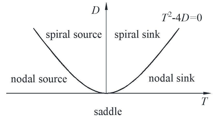
So, at point \(\left( {1,1} \right)\), this is a nonlinear system that could be center, spiral source or spiral sink.
\[\left\{ \begin{array}{l}
{x^{\prime}} = – x + xy\\
{y^{\prime}} = y – xy
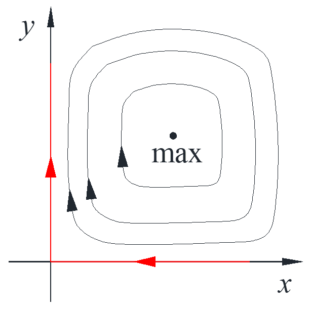
\end{array} \right. \to \frac{{dy}}{{dx}} = \frac{{y\left( {1 – x} \right)}}{{x\left( { – 1 + y} \right)}} \to \frac{x}{{{e^x}}}\frac{y}{{{e^y}}} = c\]
Integral curves are the graphs of this equation for different \(c\) contour curve of \(x{e^{ – x}}y{e^{ – y}} = c\). From physical meaning, shark dies out without any food fish, food fish grow without shark, as shown in the figure with red line and arrow. Since \(\max \left( {u{e^{ – u}}} \right) = {e^{ – 1}},\ u = 1\) and the horizontal line with particular value can only intersect twice, so the maximum point is and the curves are centers with different \(c\) values.
Effect of fishing with nets at a constant rate \(k\)
\[\left\{ \begin{array}{l}
{x^{\prime}} = – ax + bxy – kx\\
{y^{\prime}} = cy – dxy – ky
\end{array} \right. \to \left( {\frac{{c – k}}{d},\frac{{a + k}}{b}} \right)\]
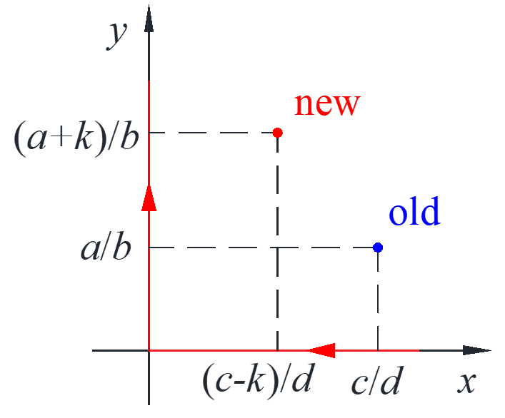
The critical point changes and actually lowering the number of shark and raising fish, this is called Volterra’s principle. The same as kill insects on trees with some poison while actually lowering the number of birds while increasing the number of insects.
1 comments On Differential equation – Part IV ODE system
I located your website from Google as well as I need to say it was a terrific
find. Thanks!