About one year ago, I tried to analyze a bolted T-stub to test the analysis method of bolted connections and verify my abaqus model referring to a journal paper, unfortunately, I could not find that paper now. Though I would not focus on steel connections in the future, I still want to make a summary of this simulation in order not to waste the effort one year ago.
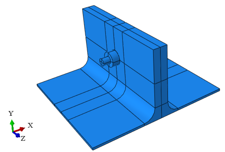
Due to the symmetry of this stub, only half is modeled as below and the whole model is symmetric about X-Z plane, which means two T stubs are connected by one bolt on each side.
Contact
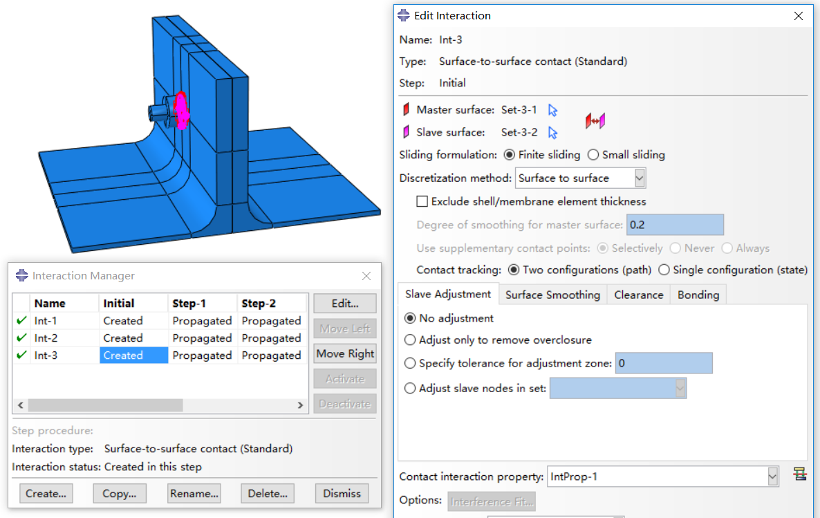
One key in this simulation is the contact between stubs and bolts. As seen below, contact property is set for the interaction between stub and stub, bolt and stub (two contact faces). Both Normal and tangential behaviors are defined with “Hard” Contact and Friction coefficient 0.3 in this simulation. This is set to define the contact during analysis, so that the elements in different instances (two T-stubs and one bolt) will not intersect with each other when they are compressed together.
Steps
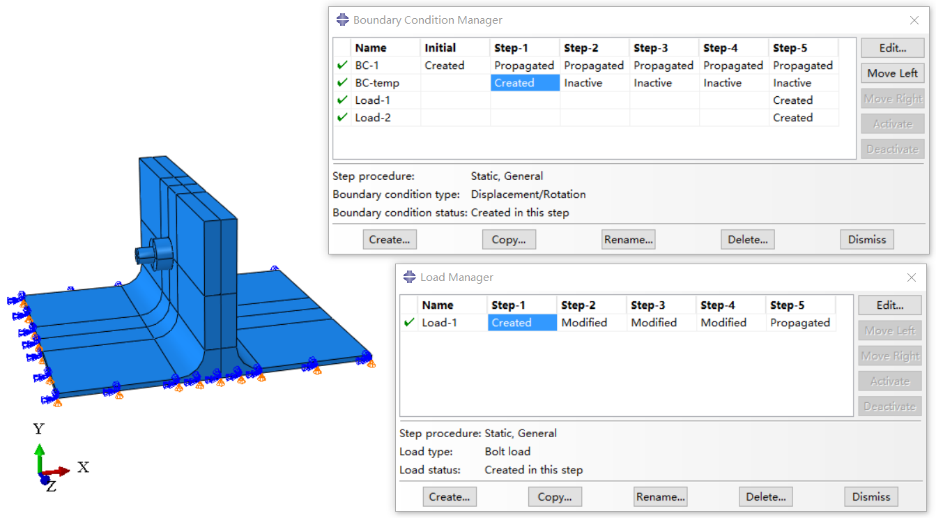
The simulation process can be summarized as below and described with the following screenshot. Totally five steps are defied with Static, General procedure.
Initial step: Apply boundary conditions. A YSYMM symmetry boundary condition is adopted here.
Step 1: Apply bolt load with a low value and define a temporary boundary condition (BC). Aim of this step is to generate some pressure between bolts and stubs, as well as stub and stub, so that no rigid displacements will be generated in next steps. You can also just apply a bolt force without apply temporary BC, but you are recommended to have a temporary BC, otherwise the analysis may result in hard convergence. Temporary BC in this simulation is zero displacements in each directions on the outer surface of nut (Y-Z plane) so that the bolt cannot move during this step..
Step 2: Inactive the temporary BC and remain the applied bolt load.
Step 3: Increase the bolt load to the value you want. This step is to simulate the bolt load acting on the stubs. The value of bolt load is normally the bolt pretension which can be chosen according to codes.
Step 4: Modify the method of bolt load to ‘Fix at current length’. This means you have tightened the bolt, which will remain the ‘same’ during life cycle of bolted T-stub.
Step 5: Apply loads or displacements to T stubs. This is the final step to simulate the force on bolted T-stub. In this simulation, two equal displacements (X direction and reversed X direction) are applied on stubs at upper section (Y-Z plane).
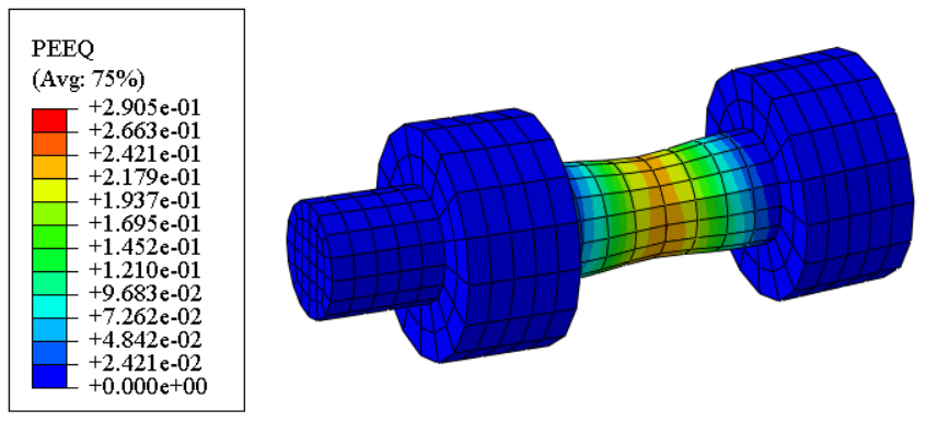
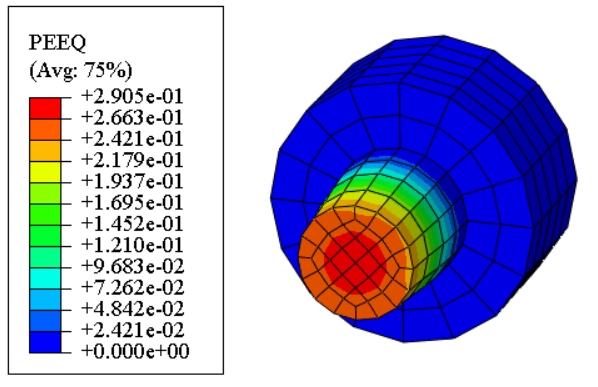
Results
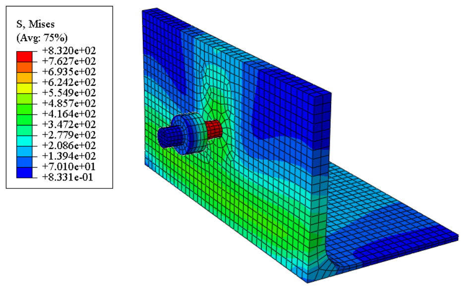
To have a better view of the results, only part of the model are selected to be displaced. The stress contour of one stub and one bolt, the PEEQ contours of bolt and middle section of nut are shown respectively. Due to none plastic strain on stubs, stubs are removed from PEEQ contours.
1 comments On Simulation of a bolted T-stub with ABAQUS
Amazing blog!