I am recently using the dynamic analysis in Abaqus, so I decided to summarize the understanding of time and amplitude in it so that I can refer to this article later if needed.
Time
- Step Time: the time period in *STEP definition.
- Total Time: the sum of all the Step Time.
- Natural time: actual time that one thing takes.
- The time in Abaqus/Standard does not have any actual meaning, it can be understood as the relative time.
- The time in Abaqus/Explicit is the actual time, that is the time that loads applied on the structure.
Amplitude definition
- Select Step time for time that is measured from the beginning of each step.
- Select Total time for total time accumulated over all non-perturbation analysis steps.
An example in ABAQUS
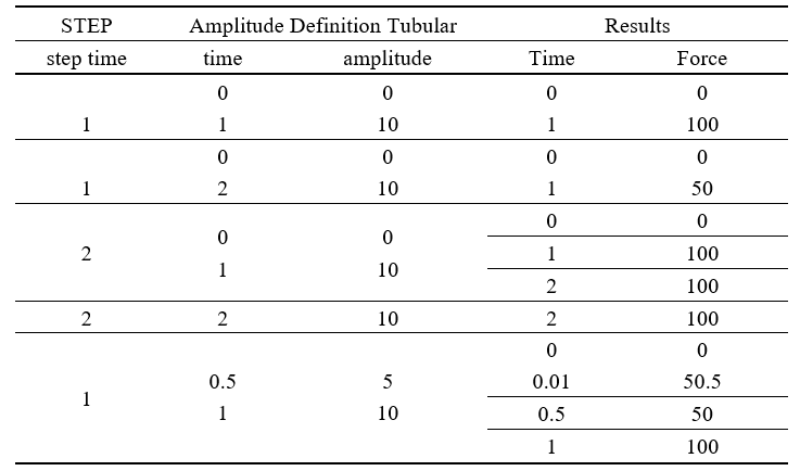
A steel frame loaded with one point load with the value 10, the Step time and Amplitude definition with Tubular is listed in the following table. The results of time and force are also listed.
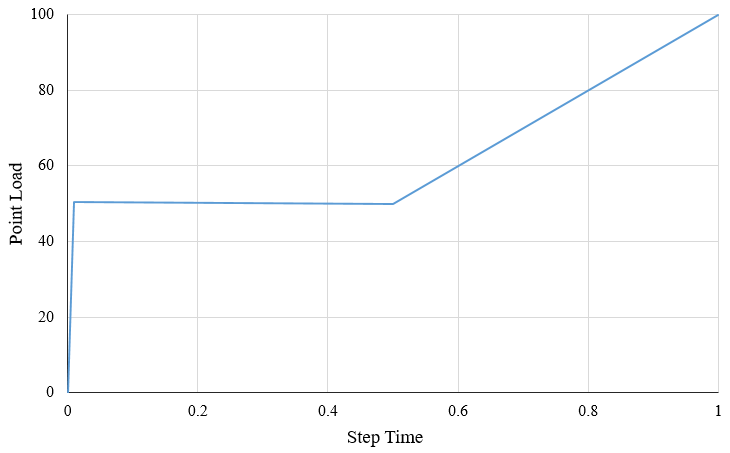
The Point Load – Step time curve of the last circumstance is illustrated below. The point load is applied up to 5 times the defined load to structure instantly, the curve at point (0.01, 50.5) is just the 0.01 times the defined load plus the 5 times the defined load.
It can be concluded that:
- Abaqus always analyzes the structure to the end of the step time.
- The time in Amplitude definition is the same meaning with step time and only the role of it is to definite the curve of applied force with the step time.
- If you didn’t define the time before or after the time in Amplitude definition, the amplitude is considered the same with the closest time.
The conclusions accord with the explanation in Abaqus Analysis User’s Guide.
About the unit of time
You can use the International System of Units and the units derived from them for all the structure, that is
- Length: m (meter)
- Mass: kg (kilogram)
- Time: s (second)
- Force: N = kg*m/s2 (Nowton)
- Pressure: Pa = N/m2 (Pascal)
- Energy/Work: J = N*m (Joule)
- Angle: rad = m*m-1 (Radian)
If you set some units associated with time as a unit different from International Unit, then the unit of time in your analysis is the unite derived from your unites. (individual understanding)
4 comments On Time and Amplitude in ABAQUS
Hi,
I have an FEM model and and I’m performing an analysis on that model with two solvers: Abaqus/Standard and Abaqus/Explicit. I need system response at each point in actual time and as you mentioned, Abaqus/Explicit is capable of doing that. But the problem is that Abaqus/Standard is very much faster than Abaqus/Explicit in simulation. Is there any way to get analysis output at every actual time-step using Abaqus/Standard?
Thanks
Hi Sajjad,
Do you need to consider dynamic effects for your model? If so (from my understanding you might need), you need to use Abaqus/Explicit. Dynamic analysis usually requires small time increments for convergence. If not, you can use Abaqus/Standard with fixed increment and output results every one step. Abaqus/Standard cannot do analysis at actual physical time since it is static analysis with governing equation KU=F (as seen not involving any physical time).
I think you can try larger time increment in Abaqus/Explicit as long as you can get satisfying results (almost the same as the results you get with very small increment).
Hope this help.
Hi and thanks for your reply.
Actually I’m a bit confused about these solvers. Let’s say I’m doing a dynamic analysis so that an equation of the following form must be solved for x(t):
M*x\ddot + C*x\dot + Kx = u(t)
Where u(t) is a general time-dependent force term. As I understand, Implicit and Explicit solvers are two types of numerical “techniques” to solve such an equation. Therefore x(t) obtained from both solvers should be the same assuming same fixed increment is used with no convergence issues. In this case, t, is the actual/physical time for both simulation.
I’d love to know your thoughts on this matter.
Hi Sajjad,
You are exactly correct! For dynamic problems, any techniques for ODE would work. Explicit solvers do not require iterations as implicit solvers since it ‘goes forward’ directly, but they usually requires smaller time increments. It is highly possible for the results from the two solvers with same increment differ each other due to the tolerances and time increment size. Usually, implicit solvers could give more stable and more accurate results as it iterates to minimize the ‘residuals’.